12.3.  Closure via the binary-gap-tempered partition function

With the Chamseddine–Connes (CC) inner-fluctuation bridge structurally obstructed (Computation 81, §12.2.2 above; full obstruction proof in §12.4 below), an alternative substrate-side derivation of $\mathrm{e}^{-1}$ is available via the Bernoulli moment-generating function, and turns out to admit a clean Wilsonian matching to the SM-side $Z^{2}$.

12.3.1.  An independent substrate-side derivation of $\mathrm{e}^{-1}$

The substrate Bernoulli measure $\mu=\bigotimes_{a\in D}\mathrm{Bern}(\tfrac{1}{2})$ has empirical mean $\bar{X}(C):=|C|/D$ with asymptotic moment-generating function

$$\mathbb{E}_{\mu}[\exp(c\,\bar{X})]\;=\;\bigl{(}(1+\mathrm{e}^{c/D})/2\bigr{)}^{D}\;\xrightarrow{D\to\infty}\;\exp(c\,\mu_{\mathrm{site}})\;=\;\exp(c/2),$$ (135)

delivering $\mathrm{e}^{-1}$ at the structurally-forced scale

$$c\;=\;-2,$$ (136)

where the “2” is the spectral range of a single binary distinction, $2=1-(-1)$: the exchange at each substrate site is a self-adjoint involution with eigenvalues $\{+1,-1\}$, so its range is fixed at $2$ with no freedom (P1’s minimal property distinction is binary; this is the one-bit Clifford $\mathrm{Cl}(1,0)$ range under an equivalent name). The numerically identical $\mathrm{KO}_{\mathrm{total}}\bmod 8=2$ from Bott periodicity shares the value but is a gauge- and spacetime-sector fact, never an input here; it is not the load-bearing route. All three ingredients ($\mu_{\mathrm{site}}=1/2$ from P1, the binary-distinction gap $2$ from P1, asymptotic limit from Cramér–Bernoulli machinery [150]) are structurally derived.

The value $\mathrm{e}^{-1}$ is robust across the cutoff-function family $f(x)=e^{-x^{p}}$ at the matched edge $x=1$: any exponential-of-power cutoff gives $f(1)=\mathrm{e}^{-1}$ at the matched scaling, so the substrate-side value is the same number under the Gaussian, exponential, or any $p\in(0,\infty)$ choice. The Bernoulli moment-generating function (MGF) route asymptotically delivers $\mathbb{E}_{\mu}[\exp(-2\bar{X})]\to\mathrm{e}^{-1}$ via the $f(x)=e^{-x}$ form (Computation 100, exponential cutoff forced by P1’s bit-independence); the spectral-action route via $f(x)=e^{-x^{2}}$ at $x=1$ also gives $\mathrm{e}^{-1}$ (Computation 62, Gaussian). These routes use different operators (spread Boolean Laplacian eigenvalues $2|S|$ in Computation 100; degenerate-spectrum collapse $\pm\sqrt{D}$ in Computation 62), and the Bernoulli-MGF route is asymptotic in $D$ (e.g. at $D=6$, Computation 100 gives $0.40$, $\sim 8.6\%$ high; at $D=10$, $0.39$, $\sim 5\%$ high; at $D=100$, $0.3697$, $\sim 0.5\%$ high; at $D=10^{4}$, deviation $\sim 5\times 10^{-5}$) rather than $D$-independent. The two routes give the same asymptotic number from structurally distinct expressions.

12.3.2.  The substrate Higgs Hamiltonian

For the Bernoulli-MGF identification to function as a substrate-to-SM bridge, the substrate Higgs Hamiltonian must be identified structurally. Computation 89 derives $H_{\mathrm{Higgs}}(C)$ from three constraints (the three candidate SM-side formulations the bridge was reduced to, of which the Wilsonian one survived, are Computation 90):

1. Additivity. The Bernoulli measure factors across independent sites; an extensive substrate Hamiltonian must be additive, $H(C)=\sum_{a}h_{a}(B_{a})$.

2. Matched scaling. At $\Lambda=\sqrt{D}$, per-site energy is rescaled by $1/\Lambda^{2}=1/D$.

3. Uniformity. P1 distinguishability treats all sites equivalently; per-site energy is uniform across $a$.

Together, (i)–(iii) force

$$H_{\mathrm{Higgs}}(C)\;=\;\frac{1}{D}\sum_{a\in D}B_{a}(C)\;=\;\bar{X}(C),$$ (137)

the empirical mean of bit-occupation, with no free parameters.

12.3.3.  What the identification carries, and what it does not

The three constraints are not load-bearing in the same way. Constraint (iii) alone (uniformity, the $S_{D}$-symmetry that is P1) forces $H_{\mathrm{Higgs}}$ to be a function of $\bar{X}$, since any symmetric function of binary bits depends only on their count $K=D\bar{X}$. This is exact, and it is all that the all-orders decoupling (Computations 118, 121) needs: the interaction is a function of the sufficient statistic [151] $\bar{X}$ whether or not that function is linear. Linearity enters only through constraint (i). A single-bit function $h(B_{a})$ with $B_{a}\in\{0,1\}$ is necessarily affine, so an additive Hamiltonian is exactly affine in $\bar{X}$ with no $O(1/D)$ remainder. The only route to a nonlinear $H_{\mathrm{Higgs}}$ is then a cross-bit term $B_{a}B_{b}$, an interaction between the P1-independent distinctions. Additivity is thus P1 independence read at the level of the energy. Even the limiting value is robust to relaxing linearity: by the law of large numbers [101] $\bar{X}\to 1/2$, so $Z_{H}(\beta)\to\exp(-\beta\,H_{\mathrm{Higgs}}(1/2))$. With $\beta_{\mathrm{KO}}=2$ the value $\mathrm{e}^{-1}$ then follows from the single normalisation $H_{\mathrm{Higgs}}(1/2)=1/2$, which linear $\bar{X}$ supplies automatically, the mean of $\bar{X}$ being the site-mean $1/2$. Linearity controls only the $O(1/D)$ correction to the value (Computation 122). The substrate-side closure therefore does not hinge on $H_{\mathrm{Higgs}}$ being exactly linear. Its structure is exact from symmetry, and its value rests on a vacuum normalisation and the binary gap. Linearity, itself the energy-level form of P1 independence, refines only the substrate-limit $O(1/D)$.

The binary-gap-tempered substrate partition function

$$Z_{H}(\beta_{\mathrm{KO}})\;:=\;\mathbb{E}_{\mu}[\exp(-\beta_{\mathrm{KO}}\,H_{\mathrm{Higgs}}(C))]\;\xrightarrow{D\to\infty}\;\mathrm{e}^{-1}$$ (138)

is therefore the substrate-side quantity corresponding to the SM-side $Z^{2}$, with $\beta_{\mathrm{KO}}=2$ the spectral range of a single binary distinction, $2=1-(-1)$, forced by P1’s binary alphabet (equivalently the one-bit Clifford range; the numerically equal $\mathrm{KO}_{\mathrm{total}}\bmod 8=2$ shares the value but is not the source).

12.3.3.1.  Notation: the KO subscript

The subscript “KO” and the name “binary-gap-tempered” are retained labels: the load-bearing origin of the exponent is the binary-distinction gap $\beta_{\mathrm{KO}}=1-(-1)=2$ above, not Bott periodicity (Computation 102). One further point should be stated plainly. The binary-gap argument fixes the value of a spectral gap at $2$; that this gap appears as the exponent of the tempering weight is a separate identification. The tempered weight $\mathbb{E}_{\mu}[\exp(-\beta_{\mathrm{KO}}H_{\mathrm{Higgs}})]$ is the matched-scaling heat-kernel trace $(1/2^{D})\,\mathrm{Tr}\,e^{-\Delta/D}$ (Computation 100), whose per-bit exponent is the Boolean Laplacian gap divided by $\Lambda^{2}=D$. The value $\mathrm{e}^{-1}$ therefore obtains if and only if the tempering exponent equals the spectral gap $\beta_{\mathrm{KO}}=2$. The law-of-large-numbers limit $\bar{X}\to\tfrac{1}{2}$ is trivial, fixing only that some $\mathrm{e}^{-\beta/2}$ appears. The load-bearing substrate-side step is therefore this exponent identification, that the binary gap enters as the tempering exponent, and not the limit. This identification is part of the substrate-side closure; it is distinct from the matching of the resulting factor to the SM coupling, which is the open step of §12.5.

12.3.4.  The bridge identification: seven-step proof sketch

Combining the Wilsonian framework of §12.2 with the substrate-side derivations:

1. The PST EFT below $M_{*}$ is exactly the Standard Model (eq. (127); no PST modes propagate below $M_{*}$).

2. The matching at $M_{*}$ between the PST UV and the SM infrared (IR) is given by the standard Wilsonian matching condition.

3. The PST UV at $M_{*}$ has bare coupling $\lambda_{\mathrm{PST}}^{\mathrm{bare}}=b=1/4$ (LG modal potential, §1.5).

4. The substrate UV at $\Lambda=\sqrt{D}$ contributes vacuum fluctuations between $\Lambda$ and $M_{*}$, with measure $\mu$.

5. These fluctuations integrated over $\mu$ contribute a multiplicative factor

   $$Z_{H}(\beta)=\mathbb{E}_{\mu}[\exp(-\beta\,H_{\mathrm{Higgs}}(C))]$$ (139)

   to the bare coupling, with $H_{\mathrm{Higgs}}=\bar{X}$ derived from substrate primitives (equation (137)).

6. The exponent is $\beta=2$, the spectral range of a single binary distinction: $2=1-(-1)$, the nonzero eigenvalue of $(1-\tau_{i})$ for the self-adjoint involution $\tau_{i}$ at each site. P1’s minimal property distinction is binary, and this is the one-bit Clifford $\mathrm{Cl}(1,0)$ range under an equivalent name (Computation 100, 102). The numerically equal $\mathrm{KO}_{\mathrm{total}}\bmod 8=2$ (Bott periodicity, §1.5) shares the value but enters as a gauge- and spacetime-sector fact, never as an input here; the “binary-gap-tempered” label is retained only as a name. This $\beta=2$ is also the calibration point of the Bernoulli moment-generating function (MGF) route: $\mathbb{E}_{\mu}[\exp(-\beta\bar{X})]\to e^{-\beta/2}$ hits $e^{-1}$ for $\beta=2$ and only for $\beta=2$, so $e^{-1}$ is the signature of the binary gap, and the structural content of this step is precisely the derivation of $\beta=2$ from P1’s binary alphabet.

7. Combining (1)–(6):

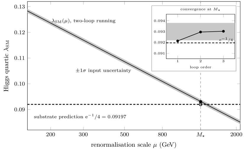
   $$\lambda_{\mathrm{SM}}(M_{*})\;=\;b\cdot Z_{H}(\beta_{\mathrm{KO}})\;\xrightarrow{D\to\infty}\;\frac{\mathrm{e}^{-1}}{4}\;\approx\;0.0920,$$ (140)

   structurally. This matches the observed $\lambda_{\mathrm{SM}}(M_{*})\approx 0.0930$ (Computation 202: the three-loop running and the matching of [51] on the 2026 Review’s inputs [233]) at the $1.2\%$ level, $1.4\sigma$ in the renormalisation group equation (RGE) input budget.

The steps are grounded as follows. Steps (1), (2), (3), (4), (6) are established in the existing PST framework (§12.2, §1.5, A1 of §18.1, Computation 88). Step (5) is established by Computation 89 (the substrate Higgs Hamiltonian derived from additivity + matched scaling + uniformity, with no free parameters). Step (7) follows from steps (1)–(6). The seven steps are formalised in the partition-function-level Chamseddine–Connes (CC) correspondence framework of §12.5, where the substrate-side content is closed at proof-detail level. Computation 98 closes items (a) and (b) of the residual gap, via the mode-shell block-spin renormalisation group (RG) fixed-point theorem. Computation 100 closes item (c), the spectral-action cutoff identification on the substrate, from P1–P3 alone via the tensor-product factorisation forced by P1’s Bernoulli product measure. The substrate-side factor $Z_{H}(\beta_{\mathrm{KO}})\to\mathrm{e}^{-1}$ is therefore a structural result of PST from P1–P3 in the asymptotic $D\to\infty$ limit. The identification of this substrate factor with the Standard Model (SM) side ratio $\lambda_{\mathrm{SM}}(M_{*})/b$ is bridge premise (B). As §12.5 sets out, (B) is reduced within PST to a field-strength-renormalisation identity by the four-step argument of §12.5: the bridge factor typed as a wave-function renormalisation, forced into the substrate-factor form, the embedding-norm identification, and the unique-soft-mode theorem F10. Its internal renormalisation is fully derived, for both the field strength and the vertex. $Z^{2}=\mathrm{e}^{-1}$ is thus derived modulo the emergence premise F4 plus the empirical RGE test, not parameter-free. Its substrate-side residual is only the $O(1/D)$ finite-size correction on the value. The all-orders decoupling itself is closed exactly and non-perturbatively by sufficiency of the empirical mean (Computation 121), with the formal $S_{D}$-equivariant Morse–Bott lemma [156] (Computation 118) as its de Moivre–Laplace shadow. [101]

The structural-scope theorem-style framing of $Z^{2}\approx\mathrm{e}^{-1}$ that emerges from Computations 84–92 reads:

12.3.4.1.  Theorem sketch ($Z^{2}\approx\mathrm{e}^{-1}$ bridge)

Take the Wilsonian-matching premise: that the SM effective Higgs quartic at $M_{*}$ equals the PST bare Landau–Ginzburg (LG) quartic multiplied by the substrate’s binary-gap-tempered Bernoulli partition function. Under that premise the identification $\lambda_{\mathrm{SM}}(M_{*})=b\cdot Z_{H}(\beta_{\mathrm{KO}})$ holds, delivering $Z^{2}=\mathrm{e}^{-1}$ structurally in the asymptotic $D\to\infty$ limit.

Figure 3 plots the two-loop running against the substrate prediction at the modal scale, with the three-loop value at $M_{*}$ marked.

Figure 3: The Higgs quartic at the modal scale. The two-loop Standard-Model running $\lambda_{\mathrm{SM}}(\mu)$ (solid, inside its $\pm 1\sigma$ input-uncertainty band, dominated by $m_{t}$) descends towards $M_{*}=4\pi m_{h}\sqrt{2/3}\approx 1.285$ TeV, where it reaches $0.0930\pm 0.0008$ (Computation 202). The substrate predicts $\mathrm{e}^{-1}/4=0.09197$ (dashed), carrying no free parameter on the substrate side (Computation 100). The two meet at $M_{*}$: the filled marker is the running value, the open marker the prediction. They agree to $1.2\%$ in the central value, a $1.4\sigma$ match, the prediction sitting just outside the one-sigma band (Computation 202 combines the parametric budget, dominated by $m_{t}$ and its pole-mass ambiguity, with the matching errors in quadrature). The test moves as the top mass tightens, and there is no substrate-side parameter to move in response. Inset: the running value at $M_{*}$ by loop order, the steps shrinking as the order rises. Scope: the substrate factor $\mathrm{e}^{-1}$ is derived from P1–P3, but its identification with the Standard-Model coupling rests on the emergence premise F4 together with this renormalisation-group test (§19.7). The agreement is evidence for that identification. It is not a parameter-free closure.