Preface

Precausal Substrate Theory
On the Nature of Reality, as I see it
Ralf Meelker
2026

First Edition

Copyright © 2026 by Ralf Meelker
All rights reserved
Authored by Ralf Meelker
Printed by Pumbo.nl BV
Published by Nashua BV

Precausal Substrate Theory
First Edition, released June 2026

Companion site	https://meelker.nl/pst
Computations	https://meelker.nl/pst/computations
Animation	https://meelker.nl/pst/animation
Video	https://meelker.nl/pst/video

ISBN 978-94-6533-774-6 (paperback)
NUR 925

Preface

In this book I pursue a single idea as far as it will go, and Precausal Substrate Theory is where it leads: that spacetime, causality, matter, and the fundamental forces are not the bedrock of reality; they arise from logic alone. The sole primitive and first postulate is property differentiation (P1), the bare capacity for distinctions to exist at all; it carries an asymmetric vector tension (P2), and when that tension crosses a threshold, modal sublimation (P3) produces instantiated geometry.

When I started, I did not set out to write a final theory, only to see whether such a precausal substrate could carry the weight physics usually places on a presupposed spacetime. It carried more than I expected. From these three postulates, together with a few natural mathematical choices and the established methods of noncommutative geometry, PST builds a common foundation beneath general relativity and quantum mechanics, recovers the Standard Model gauge structure and a three-generation count of matter, and yields one forward falsifiable prediction, a Casimir-force correction with $d^{-6}$ scaling at submicron separations, and a derived Higgs self-coupling within one sigma of the measured value (modulo the reduced bridge premise, not a separate experiment).

For transparency, the dependence of these results on the few natural choices and on noncommutative geometry is set out in full in the body, with all computations on the companion website.

The subtitle says “as I see it”, but the aim is not private: my theory is set down plainly enough that another reader can see it the same way. Most striking is how much follows from how little; I hope it encourages others to research further.

The deepest implication is also the simplest: the universe exists not because something caused it, but because a reality in which no distinctions are possible is not a reality at all.

Ralf Meelker, June 2026

Summary

Precausal Substrate Theory (PST) proposes that spacetime, causality, matter, and the fundamental forces are not the bedrock of reality; they arise from logic alone. The sole primitive and first postulate is property differentiation (P1): the capacity for distinctions to exist at all. Property differentiation carries an asymmetric vector tension (P2) as second postulate. Third postulate is modal sublimation (P3) past a Landau–Ginzburg threshold, producing instantiated geometry along the substrate’s net direction; causality is born together with geometry. These three are the theory’s only foundational postulates; the later structural results follow from them together with three extremal selection principles (minimal KO split, maximal $V_{7}$ direction algebra, maximal Dixon tensor) that are natural given P1–P3 but not derived from them (§1.7), and with the standard Chamseddine-Connes noncommutative-geometry machinery (inner fluctuations, the spectral action) applied to the substrate spectral triple that P1–P3 deliver. The field-normalisation coefficient $\mathrm{e}^{-1}$ is derived within PST in the substrate limit, and its matching to the SM coupling (bridge premise B) is reduced to a field-strength-renormalisation identity whose internal content is fully derived; it rests on the emergence of the SM as PST’s low-energy theory together with a falsifiable renormalisation-group test it passes at one sigma, not on a free parameter, so $Z^{2}=\mathrm{e}^{-1}$ is derived modulo that emergence premise rather than parameter-free.

From these three postulates a concrete mathematical structure follows. PST delivers general relativity, quantum mechanics, the Standard Model gauge group $\mathrm{SU}(3)\times\mathrm{SU}(2)\times\mathrm{U}(1)$ , fermionic matter with structural spin-statistics, and the three-generation count of matter, $N_{\mathrm{gen}}=3$ , with the Higgs identified as the projection of the substrate’s modal order parameter. The fermion mass and mixing spectrum, the Yukawa hierarchy and the CKM and PMNS matrices, is by construction not among these structural outputs. That placement is itself a theorem, not a concession: the structural layer fixed by P1–P3 is generation-symmetric at leading order, so the observed hierarchy and mixing cannot arise from it and must enter through the contingent configuration content $T(C)$ . PST predicts a Casimir correction at nanometre separations with a parameter-free, signature-distinguishable $d^{-6}$ exponent, its amplitude set by a coherence scale $d_{0}\lesssim 5.3$ nm; the $d_{0}$ -saturating scenario gives an ${\sim}10\%$ deviation at $d=50$ nm, a clean target, a null result tightening the $d_{0}$ bound rather than excluding the theory. Its other quantitative result, a derived value for the Higgs self-coupling, is consistent with the Standard Model at one sigma. Among twenty-seven surveyed substrate theories (PST and twenty-six others), PST alone delivers a pre-geometric substrate, emergent spacetime, Standard-Model gauge ingredients, and the three-generation count of matter in one framework.

The deepest implication is also the simplest: the universe exists not because something caused it, but because a reality in which no distinctions are possible is not a reality at all.

The emergence chain
The three postulates compose into a single derivation chain rather than three independent assumptions. P1 supplies a Boolean configuration space $\mathcal{P}(D)$ , the powerset of $D$ substrate sites, with cardinality $2^{D}$ , on which a Bernoulli product measure $\mu$ realises the principle of equal a priori weighting of distinctions. P2 endows $\mathcal{P}(D)$ with an asymmetric vector tension $\tau$ : each configuration carries a signed contribution $\tau(C)$ measuring its directional misalignment with the substrate’s net polarity. P3 says that when the integrated tension over a coherent region exceeds the Landau-Ginzburg threshold $\tau_{*}$ , the substrate spontaneously breaks its Boolean symmetry and crystallises a four-dimensional ring of minima. This crystallisation event is instantiated geometry: the modal angle $\theta$ becomes the (eaten) Goldstone mode whose phase aligns into the Higgs vacuum, the radial fluctuation becomes the physical Higgs scalar, and the post-sublimation manifold $M=\mathbb{R}\times S^{3}$ inherits its Lorentzian signature, its macroscopic dimension $n=4$ , and the direction of causality from the symmetry-breaking pattern. Causality is born together with geometry, not imposed on it. Everything that follows in this Summary operates within this post-sublimation manifold, with the substrate retained as the UV layer above the modal scale $M_{*}=4\pi m_{h}\sqrt{2/3}\approx 1.285$ TeV.

The Core Mathematics
The substrate is a real Connes spectral triple of KO-dimension six with sign pattern $(+,+,-)$ (Computation 3), Connes’ Lorentzian-compatible value. Its Mosco limit yields spacetime $M=\mathbb{R}\times S^{3}$ with KO-dimension four (Computation 4); the product $M\times F$ has total KO-dimension $10\equiv 2\pmod{8}$ , the Connes Standard-Model value, with the macroscopic dimension $n=4$ fixed by the minimal Connes-spectral-triple split ( $4+6=10\equiv 2\pmod{8}$ ) given the verified KO-6 substrate. The substrate’s parity grading equals the $\mathrm{Cl}(0,6)$ chirality grading $i\omega$ exactly (Computation 19), delivering the grading on which Furey’s construction rests [121]. Furey’s chain-algebra construction on $\mathbb{C}\otimes\mathbb{O}\cong\mathrm{Cl}(0,6)$ delivers $\mathrm{SU}(3)_{c}\times\mathrm{U}(1)$ on one generation of fermion content under $\mathrm{SU}(3)_{c}$ . The emergent 4-d Lorentzian Dirac sector has local Clifford algebra $\mathrm{Cl}(1,3)\cong M_{2}(\mathbb{H})$ (Cartan classification [153, 154]), so right-multiplication by $\mathbb{H}$ on the spinor module is an internal symmetry (Dixon 2010 [146], Computation 66), generating $\mathrm{Sp}(1)\cong\mathrm{SU}(2)$ . Combined via Dixon’s hyperspinor framework $T=\mathbb{C}\otimes\mathbb{H}\otimes\mathbb{O}$ , these structures synthesise to the full Standard-Model internal algebra $A_{F}=\mathbb{C}\oplus\mathbb{H}\oplus M_{3}(\mathbb{C})$ , whose unimodular unitaries are $\mathrm{SU}(3)\times\mathrm{SU}(2)\times\mathrm{U}(1)$ .

The Unified Physics
The same spectral-triple structure delivers the four otherwise-disjoint foundations of contemporary physics. General relativity: the Einstein-Hilbert action as the leading term of the Connes spectral action $\mathrm{Tr}\,f(D/\Lambda)$ , with Newton’s constant as a consistency relation among $(m_{h},M_{P},v)$ . Quantum mechanics: Mosco convergence of the Boolean Dirichlet forms with canonical commutation relations from the gradient structure and the Born rule from Gleason’s theorem. The Standard Model: gauge bosons and the Higgs as inner fluctuations of the Dirac operator on $M\times F$ , with $\phi_{\mathrm{Higgs}}=\Pi(\psi)$ , the modal condensate and the Higgs condensate are the same field at different scales. The field-normalisation factor $Z^{2}=\mathrm{e}^{-1}$ has its substrate side derived structurally from P1–P3 via tensor-product factorisation forced by P1’s Bernoulli product measure (Computation 100, §7.24). Its identification with the SM ratio $\lambda_{\mathrm{SM}}(M_{*})/b$ (bridge premise B; here $b=1/4$ is the Landau–Ginzburg modal quartic coefficient) is reduced within PST to a field-strength-renormalisation identity: the matching is a wave-function renormalisation (multiplicative, not the additive Wilsonian quartic matching), forced by P1’s product structure into the substrate-factor form, whose substrate-side value is the embedding norm of the symmetric Higgs vacuum, with a unique-soft-mode theorem (the Landau-Ginzburg order parameter is the only light field, with a spectral gap to all other substrate modes) establishing the total reduction this requires. The matching’s internal renormalisation is complete: besides the field-strength, the four-point vertex renormalisation is trivial to all orders ( $Z_{\Gamma 4}=1$ ), and this decoupling is exact, a non-perturbative consequence of the order parameter being the empirical mean of i.i.d. bits (a sufficient statistic), so $Z^{2}=\mathrm{e}^{-1}$ with no residual internal renormalisation, the only $D\to\infty$ limit being the value $\mathrm{e}^{-1}$ itself. The substrate side of $Z^{2}=\mathrm{e}^{-1}$ is derived in full; the SM-side identification $\lambda_{\mathrm{SM}}(M_{*})=b\,Z^{2}$ reduces to a single sharp, independently-testable input, the Wilsonian threshold-matching premise (the SM emerging as PST’s EFT below $M_{*}$ ), which one renormalisation-group test confirms: the predicted $\lambda_{\mathrm{SM}}(M_{*})=e^{-1}/4\approx 0.092$ sits a $\sim 0.8\%$ central-value deviation from the running SM value at full two-loop precision ( $\sim 5$ – $7\%$ at one-loop), a one-sigma match once Standard-Model input uncertainties are included, with the residual tightness set by Standard-Model RGE truncation rather than by PST. $Z^{2}=\mathrm{e}^{-1}$ is therefore parameter-free modulo that one falsifiable matching premise, not modulo any free constant. Matter: Boolean $\{0,1\}$ distinctions are fermionic occupation numbers via the CAR algebra, making spin-statistics structural. Generations: $N_{\mathrm{gen}}=3$ as the natural structural reading, three Fano-plane sub-algebras of $\mathbb{O}$ through $\hat{\tau}$ , with colour–generation distinguishability resolved conditional on the Dixon-synthesis block structure (Computation 48 and Computation 106); read structurally from Furey’s six- $\mathrm{SU}(3)$ -triplet decomposition of $\mathrm{Cl}(0,6)$ via the chain-algebra $\mathbb{C}\otimes\mathbb{H}\otimes\mathbb{O}$ .

Predictions
PST predicts a $d^{-6}$ Casimir correction at nanometre separations, a falsifiable departure from standard QFT, distinct in scaling from the $d^{-7}$ retarded Casimir-Polder regime. The Gaussian convolution-kernel form is delivered structurally by the binomial-to-Gaussian central-limit-theorem limit of the substrate’s Boolean projection kernel at matched scaling (Computation 73), with calculable $-2/(3|D|)$ correction; the coefficient $\xi=90/\pi^{2}\approx 9.12$ is the matched-scaling limit, giving the diagnostic upper bound $d_{0}\lesssim 5.3$ nm on the substrate coherence scale from current nanometre-Casimir data, a bound set precisely because PST at $d_{0}=5.3$ nm predicts $\sim$ $1\%$ at the well-measured $d=160$ nm separation, the current precision floor at that scale. At smaller separations the signal scales as $(d_{0}/d)^{2}$ : at the upper-bound $d_{0}$ the predicted correction is up to ${\sim}10\%$ at $d=50$ nm and ${\sim}64\%$ at $d=20$ nm, well outside the systematic floor of current AFM and torsion-pendulum measurements at those separations but a clean falsification target for the next-generation $1\%$ -precision programmes underway. Smaller $d_{0}$ gives correspondingly smaller corrections, but the $d^{-6}$ power-law exponent is parameter-free and signature-distinguishable from all known material corrections. The electroweak modal scale $M_{*}=4\pi m_{h}\sqrt{2/3}\approx 1.285$ TeV is a parameter-free one-loop derivation. Two structural inputs fix it: the LG modal potential at threshold has quartic coefficient $\lambda_{\mathrm{PST}}=1/4$ exactly (book §1.5), and the substrate boson–fermion mode count cancels by binomial identity ( $N_{B}=N_{F}=2^{D-1}$ ) so the only remaining contribution to $\delta m_{h}^{2}$ is the Higgs self-loop coefficient $C_{H}=6\lambda_{\mathrm{PST}}=3/2$ , giving $m_{h}^{2}=(3/2)M_{*}^{2}/(16\pi^{2})$ and therefore $M_{*}=4\pi m_{h}\sqrt{2/3}$ . The constant-function substrate vacuum mode is structurally distinct from the emergent Higgs doublet (Computations 93, 97). This is a scalar-sector result, a parameter-free one-loop derivation for the Higgs self-loop in isolation. Its extension to the full Standard Model (top, $W$ , $Z$ contributions) does not exist within PST (Computation 120): the substrate cancellation is layer-disjoint from the SM loops (Computation 105), the Veltman residual at $M_{*}$ is $\approx-3$ with no zero crossing, and the bosonic top-partner sector that would cancel it is collider-disfavoured and absent from PST’s spectrum (§7.23). $M_{*}$ is therefore irreducibly a scalar-sector prediction, a definitive bound on the scope of the result, not a closure of it. The scalar sector exhibits tree-level custodial $\mathrm{SU}(2)$ symmetry, protecting $\Delta T$ . The cosmological-constant equation of state $w=-1$ follows conditionally from the substrate’s pre-spatial framing via a steady-state-style non-dilution mechanism: the substrate’s ongoing modal sublimation contributes a time-constant energy density that does not dilute under spatial expansion, so $\dot{\rho}=0$ and the continuity equation $\dot{\rho}+3H(\rho+p)=0$ forces $w=p/\rho=-1$ exactly. The magnitude $\Lambda_{\mathrm{obs}}$ , the substrate coherence scale $d_{0}$ , the Yukawa hierarchies, and CKM mixing are contingent (they live in the realisation $T(C)$ rather than the structural P1–P3 layer) and not pinned by the postulates alone.

Standing among substrate theories
Compared against the twenty-six other substrate-style & emergent-physics theories collected in Appendix D, PST is the only entry that simultaneously (i) posits a pre-geometric substrate (finite in internal structure, not a finite universe), a Boolean distinction space rather than a presupposed infinite-dimensional arena (Wheeler superspace, a manifold, or a graph); (ii) derives spacetime as a limit theorem from that substrate via Mosco convergence of the Boolean Dirichlet form to the Laplace-Beltrami operator on $\mathbb{R}\times S^{3}$ ; (iii) derives the structural ingredients of the $\mathrm{SU}(3)\times\mathrm{SU}(2)\times\mathrm{U}(1)$ gauge group from the three postulates ( $\mathrm{Cl}(0,6)$ chain algebra delivering $\mathrm{SU}(3)_{c}\times\mathrm{U}(1)$ on one generation; $\mathrm{Cl}(1,3)\cong M_{2}(\mathbb{H})$ delivering an internal $\mathrm{SU}(2)$ on the emergent Dirac sector), with the full $A_{F}=\mathbb{C}\oplus\mathbb{H}\oplus M_{3}(\mathbb{C})$ following via Dixon’s hyperspinor synthesis; (iv) places the three-generation count of matter in Furey’s six- $\mathrm{SU}(3)$ -triplet decomposition of $\mathrm{Cl}(0,6)$ as the natural reading; and (v) contributes the derivation of a specific Standard-Model coupling value ( $\lambda_{\mathrm{SM}}(M_{*})=b\cdot\mathrm{e}^{-1}=0.0920$ at $0.8\%$ match, with the substrate-side factor $\mathrm{e}^{-1}$ derived from the foundational postulates (Computation 100); the SM-side matching reduced within PST to a field-strength-renormalisation identity whose internal content is derived, resting on the emergence premise F4 (the SM as PST’s exact low-energy effective theory below $M_{*}$ ) plus the RGE test, not inherited from the CC programme). Other entries deliver one or two of these ingredients; none delivers all five.

1. Introduction

1.1. The incompatibility of quantum mechanics and general relativity

The search for a unified account of physical reality has long been constrained by the assumption that spacetime, matter, and causal order constitute the fundamental architecture of the universe. Modern physics inherits this assumption from classical ontology, even as its two most successful frameworks, Quantum Mechanics and General Relativity, demonstrate that this assumption cannot be sustained. Quantum Mechanics describes a domain in which discreteness, nonlocality, and the breakdown of temporal sequence are intrinsic features of physical behaviour. General Relativity, by contrast, models the universe as a smooth, continuous geometric manifold whose curvature governs gravitational interaction.

These frameworks do not merely differ in mathematical form; they presuppose incompatible ontological primitives. General Relativity requires a spacetime manifold populated by loci, positions at which events occur and fields take values, and by relata, the entities that stand in geometric or dynamical relations. Quantum Mechanics, however, operates in a domain where neither loci nor relata can be taken as fundamental: superposition, entanglement, and nonlocal correlations violate the assumption that physical systems occupy definite positions or instantiate well-defined relational properties. The failure to unify General Relativity and Quantum Mechanics is therefore not a technical problem but an ontological one: each theory requires a different set of primitives. General Relativity requires loci and relata embedded in a geometric manifold; Quantum Mechanics requires a pre-geometric domain in which such constructs do not yet exist.

1.2. Assumed backgrounds and the missing question

Every physical theory, however fundamental it claims to be, begins with an implicit concession: it assumes a background. General Relativity [1] assumes a differentiable manifold and proceeds to determine its curvature. Quantum Mechanics assumes a Hilbert space evolving under a causal time parameter. String Theory and Loop Quantum Gravity [6, 7], despite their ambitions, replace one geometric background with another; strings propagate through target space, spin foam models quantize geometry but presuppose a combinatorial substrate whose relational structure is already causal in character. Even the most radical approaches to quantum gravity, including causal dynamical triangulations and causal set theory [4, 5], take causality itself as a primitive rather than a derived relation. The question that none of these frameworks address at root is the following: what is the structure that makes spacetime, causality, and the physical world possible in the first place?

This question is not merely philosophical. It has direct physical consequences. The persistent failure to reconcile Quantum Mechanics and General Relativity is not simply a technical problem of quantizing a nonlinear field theory; it is a symptom of the fact that both theories assume different things about the structure they presuppose [2, 3]. Quantum Mechanics treats time as an external parameter; General Relativity makes time dynamical. Quantum Mechanics requires a fixed causal background for the definition of states and observables; General Relativity makes the causal structure itself a dynamical variable. These are not merely different formalisms; they reflect genuinely incompatible ontological commitments about what the world is made of at its foundation. Quantum Field Theory occupies an intermediate position: it is Quantum Mechanics made compatible with special-relativistic spacetime, presupposing more background structure than QM (a fixed Minkowski metric [175] and causal order) and less than GR (no dynamical geometry). A foundational theory must derive all three; the natural demarcation is the emergence of the Lorentzian [181] action from the precausal substrate, the moment at which time-ordered products, propagators, and conservation laws first become available. A theory of quantum gravity that merely finds a way to combine QM and GR without resolving this incompatibility is not a foundational theory; it is a patch.

1.3. The precausal starting point

Precausal Substrate Theory approaches this situation differently. Rather than beginning with spacetime and asking how to quantize it, or beginning with a causal order and asking how geometry emerges, PST begins at a level prior to both: a domain in which neither geometry nor causality is defined, and in which the only primitive is the capacity for distinctions to exist.

Property differentiation is not a process, event, or transformation. It is the logical possibility of asymmetry, the condition under which difference can exist without requiring objects, relata, loci, or temporal sequence. The logical possibility of property differentiation is irreducible: any attempt to explain it presupposes it.

Once differentiation is possible, its first expression is asymmetric tension. Asymmetric tension is not a force, field, or interaction in the physical sense. It is the manifest imbalance that arises when differentiation becomes expressible. It is asymmetric without being spatial, dynamic without being temporal, structured without being geometric. Asymmetric tension is the substrate’s intrinsic asymmetry made actual, and it functions as the generative engine from which all subsequent structure emerges.

This domain, the precausal substrate, is not empty. It contains the asymmetric tension just described: a structural imbalance that arises wherever differentiated properties coexist without full symmetry. The key claim of PST is that this imbalance is not stable indefinitely. There exists a threshold beyond which the substrate cannot maintain an uninstantiated configuration, a logical boundary condition rather than a dynamical process, and when that threshold is crossed, the configuration undergoes a direct phase transition into instantiated geometry. Spacetime is not the arena in which this transition takes place. Spacetime is the transition.

1.4. The case for ontological minimality

The foundational commitment of PST is to ontological minimality. If one takes seriously the project of identifying what must exist prior to physics, prior, that is, not in a temporal sense but in the sense of logical or modal presupposition, one arrives quickly at the question of what the most primitive possible structure is. Attempts to answer this question have historically invoked points, events, fields, or relations, but all of these already carry implicit geometric, causal, or energetic content. PST makes a different choice: the minimal structure from which everything else can be derived is not a geometric entity, not a causal relation, and not a physical degree of freedom. It is simply the capacity for distinctions to exist.

To see why the historical candidates fail, consider each in turn. A point implies position: it is the primitive of location, and location presupposes a space in which positions are defined and separable. An event implies both a location and a temporal index: it is a point in spacetime, and spacetime is precisely what PST is trying to derive rather than assume. A field implies a background manifold over which it takes values, a collection of positions at each of which the field is defined; the background is assumed, not derived. A relation implies relata: two or more entities that stand in the relation, and relata are at minimum points or objects, reintroducing the geometric content that the programme aims to eliminate. Even the most abstract candidates, such as sets of abstract objects or categories of morphisms, presuppose the concept of collection or composition, which themselves rest on notions of identity and distinctness. Identity and distinctness are, in each case, the structural content that cannot be removed. PST takes this observation seriously and makes it the foundation: if every proposed primitive already presupposes the capacity to distinguish one thing from another, then that capacity is the true primitive, and the correct programme is to begin there rather than one step above it.

1.5. The foundational object: the KO-dimension-ten triple

The substrate does not, on its own, single out a number of dimensions. What it provides is an algebra of distinctions with an intrinsic involution (the complementation $C\mapsto\bar{C}$ ) and a magnitude (the tension norm). The question that fixes the structure is not how many dimensions the substrate has, but what the substrate must become for a Lorentzian quantum field theory to be definable on it. That requirement, the existence of a well-defined fermionic action continuing from the Euclidean [185] to the Lorentzian, is a demand of consistency, and it is the same demand that the incompatibility of quantum mechanics and general relativity, with which this section opened, leaves unmet by every background-assuming theory.

Connes’ noncommutative geometry [48] answers that demand with a single integer, the KO-dimension, defined modulo eight by Bott periodicity [148, 149]. It is not the dimension of any manifold; it is a property of the real structure $J$ and the grading $\gamma$ , fixing the signs of $J^{2}=\pm 1$ , $J\gamma=\pm\gamma J$ , and $JD=\pm DJ$ . Of the eight values, the canonical one for a product of spacetime with an internal space, the value at which the Euclidean fermionic action carries the sign that continues to a well-defined Lorentzian action, is KO-dimension two.

PST meets this value structurally. The substrate’s real structure has KO-dimension six (a computed result, holding for an odd number of distinction bits; §13). The Mosco limit [98] of the substrate’s Dirichlet form produces a four-dimensional Lorentzian spacetime, of KO-dimension four. KO-dimension is additive under the product, so the physical object, spacetime tensored with the substrate as its internal factor, has total KO-dimension $4+6=10\equiv 2\pmod{8}$ . Among all totals that land on the Lorentzian-compatible value two, ten is the smallest: any larger total would require a larger spacetime (which the Mosco limit does not produce) or internal structure beyond the substrate. The foundational number of PST is therefore this total KO-dimension ten, from which the four of spacetime and the six of the internal factor are the minimal split: $4+6=10\equiv 2\pmod{8}$ is the lowest sum with both summands non-negative and the total congruent to two modulo eight (the Connes Lorentzian value), given the verified parity-selected substrate KO-6 (Computation 3) and the Mosco-limit spacetime KO-4 (Computation 4). “Minimal” is therefore conditional on the parity selection but does not require an extra spectral-triple axiom beyond what Computations 3 and 4 verify; the minimality itself, and that the spacetime four is the unique mod-8 complement of the substrate six rather than an independent input, is a finite arithmetic check (Computation 128).

PST adopts three such extremal selection principles: minimal split for the KO-bookkeeping (the present paragraph); maximal directional structure for the substrate ( $V_{7}=\mathrm{Im}(\mathbb{O})$ is the largest vector part of any normed division algebra by the Hurwitz classification [164], preferred to the 3-dimensional cross product because it is the maximal norm-multiplicative vector product; §3); and maximal-tensor hyperspinor envelope for the substrate–internal-algebra synthesis ( $\mathbb{C}\otimes\mathbb{H}\otimes\mathbb{O}$ is the full Dixon tensor of all four Hurwitz division algebras, preferred to proper subalgebras such as Furey’s [121] $\mathbb{C}\otimes\mathbb{O}$ alone; §8.7). All three are natural choices given P1–P3 but none is derived from them; the recurring “forced” phrasing in the body sections should be read as “forced under the chosen extremal selection principles.”

This total has nothing to do with the ten of superstring theory. There, ten is the dimension of a smooth target manifold, fixed by cancellation of the worldsheet conformal anomaly. Here, ten is a KO-theoretic invariant, defined only modulo eight, of the real structure of a product spectral triple; it counts no spatial directions, and involves no strings, no extended objects, no worldsheet, and no anomaly to cancel. PST arrives at ten by Connes–Bott periodicity applied to a distinction-first substrate.

In this framework the instantiated geometry is four-dimensional and Lorentzian; the remaining six of the KO-bookkeeping live in a finite noncommutative internal factor with no spatial extent, the algebraic home of the gauge structure and the matter content. PST goes beyond a substrate-level grounding of the Connes-Chamseddine programme [49]: the internal algebra $A_{F}=\mathbb{C}\oplus\mathbb{H}\oplus M_{3}(\mathbb{C})$ that programme posits is, in PST, derived from the primitive distinction structure (§8.7). The substrate’s parity-selected real structure (Computation 3) delivers the Cl(0,6) chirality grading exactly (Computation 19: $\gamma_{K}=i\omega$ to machine precision in the Jordan-Wigner representation [105]), and Furey 2014 [121] calculates $A_{F}$ as the commutant of the matter representation on the resulting minimal left ideal. The remainder of this book develops the structures that follow (general relativity via the spectral action, the gauge group as the unimodular unitaries of $A_{F}$ , the matter content of one generation, and quantum mechanics), and isolates the two quantitative bounds (the reduced bridge premise B behind $Z^{2}=\mathrm{e}^{-1}$ and the negatively-settled full-Standard-Model extension of $M_{*}$ ) in §13.

The substrate–Higgs identification: two viewpoints of one field.

The substrate’s Landau–Ginzburg order parameter [8] $\psi$ and the Standard-Model Higgs field $\phi$ [75] are not two analogous objects but a single field viewed at different energy scales: $\phi=\Pi(\psi)$ , the modal condensate as seen from inside the instantiated geometry. The substrate-level LG sombrero is the same sombrero as the SM Higgs potential under the maps $\varepsilon\leftrightarrow\mu^{2}$ , $b\leftrightarrow\lambda$ , $r_{0}\leftrightarrow v/\sqrt{2}$ (doublet convention, $\lambda_{\mathrm{PST}}=\tfrac{1}{4}$ ; §1.7); the measured Higgs mass $m_{h}\approx 125$ GeV follows from the quartic via $m_{h}=\sqrt{2\lambda_{\mathrm{SM}}}\,v$ with no further input. The two viewpoints framing is developed in §10.2; its implications for electroweak symmetry breaking, the $\mathrm{U}(1)_{\mathrm{em}}$ phase as the Stueckelberg-eliminable Goldstone [163, 43], and the post-Newtonian decoupling of scalar modes appear in §8.4, §8.3, and §9.7 respectively; §12.5 situates the identification against the existing literature on electroweak symmetry breaking.

1.6. Principal consequences

The consequences of this reorientation are far-reaching. Because spacetime and the causal order it carries appear together in a single, nontemporal transition, causality is not fundamental. It is coemergent with geometry, a derived structural relation that exists only within the instantiated domain. This means that asking what caused the universe to come into being is not a deep question with a hidden answer; it is a category error. Causality did not exist prior to the transition that brought geometry, and therefore causality itself, into being. This is not an evasion of the question but its dissolution.

The same logic dissolves the Big Bang as a foundational event. The Big Bang implies a locus of origin, a privileged point in spacetime from which everything expands. But PST denies that loci are primitive. Instantiation is continuous and distributed across the substrate; it has no centre, no start, and no singular event. What cosmology calls the Big Bang is a perspectival artifact: the appearance of a beginning as seen from within an instantiated geometry that was never born at a point. The cosmological implication is not a multiverse in the conventional sense of discrete bubble universes appearing at separate loci, but something more fundamental: the substrate instantiates geometry continuously and everywhere at once, without boundaries or origins. What is called this universe is not one bubble among many; it is a region of observation within a continuous, unbounded field of instantiation.

A third consequence concerns orbital motion and gravitational structure. The standard representation of gravitational attraction, the rubber sheet or elastic membrane of General Relativity pedagogy, depicts spacetime as a funnel-shaped surface with a single minimum. In that picture a stable orbit requires a precisely tuned tangential velocity, which must be imposed on the geometry as an external initial condition; the geometry itself cannot explain where it comes from. This is not merely a deficiency of the pedagogical analogy. In General Relativity proper, orbital motion is described as geodesic motion in curved spacetime, and the geodesic equation correctly determines the shape of any path through a given metric. But which geodesic a body follows, whether circular, elliptical, or radially infalling, remains an initial condition that General Relativity takes as given. The metric determines the available paths; it cannot explain why a body is on one path rather than another. The vacuum that emerges from modal sublimation is structurally different. Below the threshold, the modal potential has not one minimum but a ring: the set of all configurations that minimise the potential at equal tension. Motion along this ring is not a special assumption; it is the only stable state available to any instantiated configuration. Circular orbital motion, from the orbital motion of subatomic particles to planetary orbits to galactic rotation to the spin of black holes, is therefore not a mechanical accident or a lucky initial condition in PST. It is a structural consequence of the topology of the vacuum manifold. General Relativity describes orbital mechanics correctly at macroscopic scales but cannot derive the existence of orbital motion from first principles; PST does.

At the moment of instantiation, when tension first crosses the modal threshold, the substrate’s algebraic structure organises itself into two qualitatively different pieces. The Mosco limit of the Boolean Dirichlet form produces a four-dimensional Lorentzian spacetime $M=\mathbb{R}\times S^{3}$ directly; there is no ‘dimensional reduction’ from a higher-dimensional manifold. Separately, the substrate’s internal algebraic content is the finite noncommutative factor $A_{F}=\mathbb{C}\oplus\mathbb{H}\oplus M_{3}(\mathbb{C})$ , an algebraic object with no spatial extent. This algebra identity follows under Dixon’s hyperspinor synthesis of the substrate’s $\mathrm{Cl}(0,6)$ chain algebra and the emergent spacetime’s $\mathrm{Cl}(1,3)\cong M_{2}(\mathbb{H})$ Dirac-spinor [23] algebra (Cartan classification of real Clifford algebras [153, 154]), both delivered by P1–P3 in conjunction with the Connes-spectral-triple framework. The principal pieces (§8.7), three verified computations and one literature construction, are: Computation 3, the substrate’s parity-selected real structure on an odd number of distinction bits delivers $\gamma_{K}^{2}=+I$ with the Connes Lorentzian KO-6 sign triple $(\varepsilon,\varepsilon^{\prime},\varepsilon^{\prime\prime})=(+,+,-)$ ; Computation 19, $\gamma_{K}$ equals the $\mathrm{Cl}(0,6)$ chirality grading $i\omega$ exactly in the Jordan-Wigner representation, so the chirality projector $f=(I+i\omega)/2$ is delivered directly by the substrate; Furey 2014 [121] chain-algebra construction on the resulting minimal left ideal delivers $\mathrm{SU}(3)_{c}\times\mathrm{U}(1)$ on one generation of fermion content; and Computation 66, the emergent Lorentzian Dirac sector $\mathrm{Cl}(1,3)\cong M_{2}(\mathbb{H})$ supplies the $\mathbb{H}$ factor of $A_{F}$ via right- $\mathbb{H}$ -multiplication on the spinor module (Dixon 2010 [146]). The algebra identity holds, with no appeal to the Chamseddine-Connes-Marcolli classification [50]. The foundational object PST identifies is the product of $M$ and $F$ , a real spectral triple of total KO-dimension ten, whose $4+6=10$ minimal split compatible with a Lorentzian fermion action is derived above (§1.5).

Furthermore, because both General Relativity and Quantum Mechanics emerge as projections of the same precausal structure, with the first operating at macroscopic scales of tension and the second near the threshold where configurations are only marginally instantiated, their unification is not a matter of quantizing one and deforming the other. It is a matter of recognizing that they describe the same underlying reality from different regimes of a single precausal parameter. Work on emergent gravity [18, 19] has approached this question from within the instantiated domain; PST proposes the precausal domain as the natural resolution point.

1.7. The foundational postulates of PST

The theory is formulated using a Landau-Ginzburg variational principle for the modal threshold [8] and a categorical functor for the sublimation map [9], with an explicit tension-to-metric construction that derives the Minkowski signature rather than postulating it. Its principal falsifiable prediction is a Casimir correction with $d^{-6}$ scaling [11, 12, 13, 14, 15] and coefficient $\xi=90/\pi^{2}$ (parameter-free under the Gaussian projection-kernel choice; the $d^{-6}$ exponent is kernel-independent, derived in Computation 139), with diagnostic amplitude $\xi d_{0}^{2}$ measurable at submicron plate separations (§10).

PST rests on three independent foundational postulates (P1–P3). A fourth formal statement, the Laplace-type projection condition, is not postulated: it is reduced to P1–P3 via Mosco convergence of Boolean Dirichlet forms (§7.6) under A1–A7; the equidistribution condition A3, the single named inequality $\eta_{K,R}<d_{0}^{2}/4$ , is supplied by P3’s maximum-entropy sublimation, so the Mosco limit is unconditional (under P1–P3) and equicoercivity A7 follows as an unconditional theorem (§7.7); the Laplace-type projection statement is given separately below for ease of reference. The postulates are stated in terms of a direction algebra $V_{7}$ , the 7-dimensional vector space over $\mathbb{R}$ equipped with the octonion vector product.

P1 (The Distinction Primitive, with directional content).

There exists a nonspatiotemporal set $D$ of primitive properties. Each property $a\in D$ carries inherent directional content $v(a)\in V_{7}$ . The substrate is the structure $(D,\delta,v)$ where: (i) $\delta$ is the symmetric irreflexive distinction relation, and (ii) $v\colon D\to V_{7}$ is the direction assignment. The dimension $7$ of $V_{7}$ is not chosen: by Hurwitz’s classification, the only normed division algebras over $\mathbb{R}$ are $\mathbb{R}$ , $\mathbb{C}$ , $\mathbb{H}$ , $\mathbb{O}$ , of total dimension $1,2,4,8$ ; their vector parts (orthogonal complements of the identity) have dimensions $0,1,3,7$ . The maximal vector dimension compatible with norm-multiplicativity is therefore $7$ , realised uniquely by the octonion vector product on $V_{7}$ , and we adopt this maximal direction algebra as the carrier of directional content. No geometric, causal, or temporal structure is presupposed; the directional content in $V_{7}$ is the only structural enrichment of bare distinguishability.

P2 (Asymmetric Vector Tension).

The tension functional $T\colon\mathcal{P}(D)\to V_{7}$ is $V_{7}$ -valued. It is asymmetric under complementation: $T(D\setminus C)\neq-T(C)$ generically. Equivalently, the total substrate tension $T(D)$ does not vanish; it provides a substrate-level directional bias in $V_{7}$ . This bias is the source of the preferred direction $\hat{\tau}=T(D)/|T(D)|$ that is selected at modal sublimation. Asymmetric vector tension is the sole source of directedness, including the chiral direction that organises both the colour gauge group and the generation count (§8.15).

P3 (The Landau–Ginzburg Modal Potential on $V_{7}$ ).

The order parameter $\psi\colon\mathcal{C}\to V_{7}$ is $V_{7}$ -valued. Its dynamics near the modal threshold are governed by the $G_{2}$ -invariant Landau–Ginzburg functional

\mathcal{F}[\psi,\varepsilon]\;=\;\int_{\mathcal{C}}\!\left[-\varepsilon\,% \langle\psi,\psi\rangle+\tfrac{1}{4}\langle\psi,\psi\rangle^{2}+c\,|\nabla_{% \mathcal{C}}\psi|^{2}_{V_{7}}\right]d\mu,

(1)

where $G_{2}=\mathrm{Aut}(\mathbb{O})$ is the automorphism group of the octonion product (which acts on $V_{7}$ in its 7-dim irreducible representation), $\langle\cdot,\cdot\rangle$ is the canonical inner product on $V_{7}$ , and $\varepsilon=|T(C)|-\tau$ is the scalar excess tension. We adopt throughout the doublet convention: the quartic coefficient $\tfrac{1}{4}$ is the coefficient of the doublet bilinear $\langle\psi,\psi\rangle^{2}$ , identified at the matched scale with the Standard-Model doublet form $V_{\mathrm{SM}}=\lambda_{\mathrm{SM}}(\Phi^{\dagger}\Phi)^{2}$ via $\langle\psi,\psi\rangle\leftrightarrow\Phi^{\dagger}\Phi$ (not the real-component norm; the two differ by a factor of two). In this convention $b=\lambda_{\mathrm{PST}}=\tfrac{1}{4}$ is the coefficient of $(\Phi^{\dagger}\Phi)^{2}$ , the same convention as $\lambda_{\mathrm{SM}}$ , so that the field-normalisation ratio $Z^{2}=\lambda_{\mathrm{SM}}(M_{*})/b$ is a ratio of two same-convention couplings (§7.23, Computation 109). Under the radial reduction $\langle\psi,\psi\rangle\to\psi^{2}$ the postulate collapses to the scalar form $-\varepsilon\psi^{2}+\tfrac{1}{4}\psi^{4}$ of equation (23). The gradient term is the Boolean Dirichlet form on $\{0,1\}^{D}$ extended pointwise on $V_{7}$ values:

|\nabla_{\mathcal{C}}\psi|^{2}_{V_{7}}\;\equiv\;\sum_{\begin{subarray}{c}C,C^{% \prime}\in\{0,1\}^{D}\\ |C\triangle C^{\prime}|=1\end{subarray}}\langle\psi(C)-\psi(C^{\prime}),\,\psi% (C)-\psi(C^{\prime})\rangle.

(2)

The potential admits a continuous family of degenerate minima at $|\psi|=r_{0}(\varepsilon)$ parameterised by the unit direction $\hat{\psi}\in S^{6}\subset V_{7}$ . Modal sublimation locks $\hat{\psi}$ to $\hat{\tau}=T(D)/|T(D)|$ , not by spontaneous symmetry breaking, but by direct determination from the substrate’s directional bias (P2).

Modal sublimation instantiates the maximum-entropy ( $\mu$ -typical) configuration consistent with the tension data: among the substrate configurations that cross the threshold, the realised one carries no unforced density structure beyond what $T$ determines. This maximum-entropy selection is a typicality property of sublimation, internal to P3 and not a fourth postulate; its role is to fix the realised emergence cloud as the equidistributed one, so that the equidistribution condition A3 of the Mosco limit (§7.7, §4.11) holds as a consequence of P3 rather than as an added premise.

Derived statement: the Laplace-type projection. The projection kernel $\widetilde{K}(x,y;t)$ is, to leading order in $t$ , the heat kernel of a Laplace-type operator $\Pi(L)$ on $L^{2}(M,\mathrm{dvol}_{g})$ whose principal symbol is the emergent metric:

\Pi(L)\;=\;-g^{\mu\nu}\nabla_{\mu}\nabla_{\nu}\;+\;(\text{lower order}),

(3)

so that $\widetilde{K}(x,y;t)=\langle x|e^{-t\Pi(L)}|y\rangle$ . This statement is not postulated: it follows from P1–P3 by Mosco convergence of the $V_{7}$ -valued Boolean Dirichlet form to the standard Laplace–Beltrami form [169] on $M=\mathbb{R}\times S^{3}$ along the selected direction $\hat{\tau}$ (§7.6). Structurally PST rests on three independent postulates only.

The complex-scalar Landau–Ginzburg formulation is a 2-dimensional slice of the present $V_{7}$ -formulation: choosing any 2-plane $\mathbb{C}_{\hat{\tau},\hat{\eta}}\subset V_{7}$ spanned by $\hat{\tau}$ and a perpendicular unit direction $\hat{\eta}\perp\hat{\tau}$ projects the present potential to the familiar complex-scalar form $\mathcal{F}_{\mathbb{C}}[\psi_{\mathbb{C}},\varepsilon]$ with $\psi_{\mathbb{C}}=\langle\psi,\hat{\tau}\rangle+i\,\langle\psi,\hat{\eta}\rangle$ . The ring-of-minima $S^{1}$ vacuum manifold of the scalar formulation is the projection of the $S^{6}$ vacuum manifold to that 2-plane. All quantitative predictions involving the scalar-formulation ring are preserved under the projection; the additional 5 directions perpendicular to $\mathbb{C}_{\hat{\tau},\hat{\eta}}$ carry the gauge-theoretic content (colour $\mathrm{SU}(3)$ and the three generations, §8.15).

The Bernoulli measure [168] $\mu=\bigotimes_{a\in D}\mathrm{Bern}(\tfrac{1}{2})$ is not a postulate; it is the unique measure on $\mathcal{P}(D)$ invariant under relabelling and under per-property complementation (§2.5). The Lorentzian signature $(+,-,-,-)$ is derived from hyperbolic well-posedness of the Goldstone wave equation along $\hat{\tau}$ (Computation 2). See §13 for the full accounting and for the open research that remains.

1.8. Structure of this book

The remainder of this book develops PST in full. Chapter 2 develops postulate P1 (property differentiation) with its mathematical expression. Chapter 3 develops postulate P2 (asymmetric vector tension). Chapter 4 develops postulate P3 (modal sublimation): the modal threshold and its variational formulation in the first half, and the sublimation transition formalised as a categorical functor with explicit construction in the second half. Chapter 5 addresses the coinstantiation of spacetime and causality. Chapter 6 consolidates the emergence chain. Chapter 7 derives energy, matter, and fields as projections of asymmetric tension, and establishes the equicoercivity A7 as an unconditional theorem, its equidistribution condition A3 (the closure margin $\eta_{K,R}<d_{0}^{2}/4$ below which the continuum manifold limit closes, for the emergence-determined realisation $\rho_{n}$ ) supplied by P3’s maximum-entropy sublimation (§7.7). Chapter 8 derives the Standard Model gauge group from the internal algebra $A_{F}=\mathbb{C}\oplus\mathbb{H}\oplus M_{3}(\mathbb{C})$ (closing the Conjecture-1 algebra identity, §8.7), fixes the hypercharge assignment, and establishes gauge anomaly cancellation as a structural theorem. Chapter 9 develops the physical predictions of the theory, including a quantitative Casimir correction. Chapter 10 grounds Newton’s constant [174] as the gravitational term of the spectral action and identifies the discreteness scale $d_{0}$ with the Landau-Ginzburg coherence length of the modal vacuum, establishing the Casimir correction (the $d^{-6}$ scaling is a necessary signature; the parameter-free coefficient $\xi=90/\pi^{2}$ fixes the diagnostic amplitude $\xi d_{0}^{2}$ that selects PST) as a concretely detectable experimental signal. Chapter 11 develops PST’s cosmology: the Friedmann [68] equations are derived, the Cosmological Principle is established as a theorem of the Bernoulli measure, and ongoing instantiation is shown to deliver the equation of state $w=-1$ structurally, conditional on the substrate’s pre-spatial framing (§7.17). Chapter 12 positions PST in relation to existing frameworks. Chapter 13 catalogues the structural and mathematical research problems that the theory resolves, sector by sector. Chapter 14 concludes. Appendix A is a consolidated table of the symbols recurring through the book, grouped by sector, each with the section where it is first introduced. Appendix B is the register of the computation scripts cited throughout as Computation $N$ ; Appendix C consolidates the status of every substantive claim of the book; Appendix D tabulates the comparison to other substrate and emergent-physics theories; Appendix E collects the bibliographic references.

1.9. Summary

Physics has produced two extraordinary theories: General Relativity, which describes how gravity shapes space and time, and Quantum Mechanics, which governs the behaviour of subatomic particles. Both are spectacularly accurate in their respective domains. But they rest on incompatible assumptions about the nature of reality, and every attempt to merge them has stalled at the same conceptual barrier. This book argues that the problem is not merely technical but ontological: both theories assume a background they cannot explain. Precausal Substrate Theory resets the starting point to something deeper, the bare capacity for distinctions to exist, and derives spacetime, gravity, and quantum fields from there.

2. Property Differentiation

2.1. Property differentiation

A property is differentiated from another not by virtue of occupying different positions in space or occurring at different times (positions and times do not yet exist), but simply by being other. Two properties are differentiated if and only if they are not identical. Nothing further is required: no metric distance, no causal connection, no ordering relation, no extensional structure of any kind. Property differentiation is the minimal condition under which the concept of a distinction is meaningful, and it is the sole primitive of the precausal substrate.

The concept of otherness that this definition invokes is purely logical. It is the primitive of non-identity: $a$ is other than $b$ if and only if it is not the case that $a=b$ . This does not require the two properties to be distinguishable by any observer, separable in any physical sense, or related by any causal or spatial connection. It requires only that identity fails. Two properties that are distinct in this sense need share nothing beyond their mutual non-identity; they carry no further structure, no mass, no charge, no location, no duration. The precausal substrate is therefore a domain in which the only thing that is true is that some properties are not the same as others. All of physics, in the PST programme, must be derivable from that single fact.

This choice of primitive is not arbitrary, and it is not merely the result of a preference for minimality. It is the result of asking what must be true of any domain that is to give rise to structure at all, and then identifying the unique weakest condition that satisfies the requirement. The requirement is this: a domain from which structure can emerge must be capable of nontrivial differentiation. If every element of the domain were identical to every other, the domain would be featureless and nothing could arise from it. Property differentiation is precisely the weakest condition under which nontrivial differentiation is possible. It is weaker than any spatial, causal, or metric structure, and it is not derivable from anything weaker than itself: any domain that contains less structure than property differentiation contains no nontrivial distinctions at all and is, in effect, the null domain from which nothing can arise. Property differentiation is therefore not merely minimal; it is the unique minimal structure with the required generative capacity. The substrate is genuinely precausal: it exists in a mode of being in which causality has no purchase, because causality requires a temporal ordering of events, and temporal ordering requires positions and durations, neither of which are available at this level.

2.2. The substrate triple $(D,\delta,v)$

The substrate is the triple $(D,\delta,v)$ :

•

$D$ is a set of primitive properties.
•

$\delta\colon D\times D\to\{0,1\}$ is the distinction relation, symmetric and irreflexive:

$\displaystyle\delta(a,b)$ $\displaystyle\;\implies\;\delta(b,a)$ (4)

$\displaystyle\neg\,\delta(a,a)$ (5)
•

$v\colon D\to V_{7}$ is the direction assignment: each property $a\in D$ has inherent directional content $v(a)\in V_{7}$ in the 7-dimensional direction algebra.

No further axioms are imposed on $\delta$ . There is no transitivity requirement, no totality requirement, no metric on $D$ , no topology, and no ordering. The direction assignment $v$ replaces a labelled-set structure with a $V_{7}$ -vector content; without it, distinctions would carry magnitude only (“this property is distinct”) with no record of what kind of distinction. With $v$ , each distinction is a vector in the maximal Hurwitz direction algebra, structured by the octonion vector product.

2.3. The direction algebra $V_{7}$

$V_{7}\cong\mathbb{R}^{7}$ as a vector space, equipped with:

•

a positive-definite inner product $\langle\cdot,\cdot\rangle$ ,
•

a bilinear vector product $\times\colon V_{7}\times V_{7}\to V_{7}$ satisfying $\langle u\times v,u\rangle=\langle u\times v,v\rangle=0$ and $|u\times v|^{2}=|u|^{2}|v|^{2}-\langle u,v\rangle^{2}$ .

This is the unique 7-dimensional algebra satisfying these properties (Hurwitz); equivalently, it is the vector part of the octonions $\mathbb{O}$ under octonion multiplication. The automorphism group of $V_{7}$ (preserving both the inner product and the vector product) is the exceptional Lie group $G_{2}$ , of real dimension $14$ . The choice of dimension $7$ for the direction algebra is forced: no other dimension supports a maximal normed-product structure over $\mathbb{R}$ .

2.4. Configurations and configuration space

A configuration $C\subseteq D$ is a collection of properties considered jointly. The space of configurations is $\mathcal{C}=\mathcal{P}(D)$ . The total direction content of a configuration is the sum

v(C)\;=\;\sum_{a\in C}v(a)\;\in\;V_{7}.

(6)

This is the natural $V_{7}$ -valued aggregate of the directional content of the properties in $C$ . The asymmetric tension functional of P2 is structurally related to (but distinct from) $v(C)$ : $T(C)$ encodes the magnitude and directional bias of the configuration’s tension, with the magnitude governing modal sublimation and the direction inheriting from $v$ via the asymmetric tension construction of §3.

It is within the configuration space $\mathcal{C}$ that the modal structure of PST is expressed. These are not temporal dynamics; they concern what is possible, what is necessary, and what cannot remain uninstantiated.

2.5. The canonical measure on configurations

Before assembling the functional (§4), the measure $\mu$ on $\mathcal{C}$ must be fixed. The variational formulation demands integration over all configurations, and the choice of measure is not arbitrary: it must follow from the structure of $(D,\delta)$ alone, without invoking any geometric, probabilistic, or metric primitive that would introduce a new assumption at the level of the substrate.

The configuration space $\mathcal{C}=\mathcal{P}(D)$ is the power set of $D$ : the collection of all subsets of the property domain. The structure $(D,\delta)$ carries a natural symmetry group, its automorphism group $\mathrm{Aut}(D,\delta)$ , consisting of all bijections $f:D\rightarrow D$ that preserve the distinction relation: $\delta(a,b)\iff\delta(f(a),f(b))$ for all $a,b\in D$ . Every such automorphism lifts canonically to a bijection on $\mathcal{C}$ by acting elementwise: $f\cdot C=\{f(a):a\in C\}$ . Since the only primitive is $(D,\delta)$ , and since the definition of a configuration is simply a subset of $D$ , the measure $\mu$ must be invariant under this lifted action: no configuration should receive more weight than any automorphically equivalent configuration.

The key observation is that in the precausal substrate, all properties in $D$ are structurally equivalent: the distinction relation $\delta$ is irreflexive and symmetric but otherwise unconstrained, so there is no intrinsic difference between any one property and any other beyond their bare identity. No property is marked, distinguished, or preferred. This means that the full symmetric group on $D$ is contained in $\mathrm{Aut}(D,\delta)$ as a subgroup: any permutation of $D$ is an automorphism, since $\delta$ treats all pairs equally. A measure invariant under all permutations of $D$ is invariant under all relabellings of the properties, which is the minimal requirement for a measure that introduces no additional structure beyond $(D,\delta)$ .

For a finite domain $D$ of cardinality $n$ , the canonical measure on $\mathcal{P}(D)$ is the uniform measure, assigning equal weight to all $2^{n}$ subsets:

\mu(C)=2^{-n}\qquad\text{for all }C\in\mathcal{C}

(7)

Permutation invariance alone does not force this: any weighting that depends only on the cardinality $|C|$ is permutation-invariant. What forces it is the per-property form of complementation invariance. The primitive $(D,\delta)$ draws no distinction between the presence and the absence of each individual property, so for every $a\in D$ the single-property flip $\sigma_{a}\colon C\mapsto C\mathbin{\triangle}\{a\}$ is a symmetry of the substrate. The group generated by the flips acts transitively on $\mathcal{P}(D)$ , so the unique flip-invariant probability measure is the uniform one; permutation invariance then holds automatically.

For an infinite domain $D$ , the natural extension is the Bernoulli product measure $\mu=\bigotimes_{a\in D}\mathrm{Bern}(1/2)$ , the unique probability measure on $\{0,1\}^{D}$ invariant under all permutations of the index set $D$ and under every single-property flip $\sigma_{a}$ (the flips act transitively on every finite cylinder, forcing the uniform marginal on each finite window; Kolmogorov extension then gives the product measure):

\mu\bigl{(}\{C\in\mathcal{C}:C_{0}\subseteq C\}\bigr{)}=2^{-|C_{0}|}\qquad% \text{for all finite }C_{0}\subseteq D

(8)

This is the projective limit of the uniform measures on all finite sub-domains of $D$ .

The value $1/2$ for the Bernoulli parameter is not arbitrary: it is the unique value for which $\mu$ is invariant under complementation, $C\mapsto\bar{C}=D\setminus C$ . Complementation invariance is required by the structure of property differentiation: the distinction relation $\delta(a,b)$ is symmetric, and no configuration is intrinsically more natural than its complement. A configuration $C$ and its complement $\bar{C}$ represent exactly the same collection of pairwise distinctions, viewed from two opposite orientations that are not distinguished by anything in $(D,\delta)$ . Assigning $\mu(C)\neq\mu(\bar{C})$ would introduce a polarity into the substrate that has no basis in the primitive. The Bernoulli parameter $1/2$ is therefore forced by complementation invariance alone, independently of the permutation argument.

The derivation may be summarised as a theorem.

Theorem (Canonical Measure). Let $(D,\delta)$ be a precausal property domain with $\delta$ symmetric and irreflexive. The unique probability measure $\mu$ on $\mathcal{C}=\mathcal{P}(D)$ that is (i) invariant under all automorphisms of $(D,\delta)$ and (ii) invariant under every single-property complementation $\sigma_{a}\colon C\mapsto C\mathbin{\triangle}\{a\}$ , $a\in D$ (the global complementation $C\mapsto\bar{C}$ is their composition), is the Bernoulli product measure $\mu=\bigotimes_{a\in D}\mathrm{Bern}(1/2)$ .

The proof is immediate from (ii) alone: the group generated by the single-property flips acts transitively on $\mathcal{P}(D)$ for finite $D$ , and on every finite cylinder for infinite $D$ , so an invariant measure weights all configurations (all cylinders over a given window) equally, which is the Bernoulli product measure; (i) then holds automatically. Condition (ii) is the exact measure-theoretic expression of P1’s symmetry between the presence and the absence of each distinction. The per-property form is essential: global complementation together with permutation invariance would not suffice (a mixture supported on $\{\emptyset,D\}$ satisfies both), which is why the flip invariance is the honest hypothesis.

The measure $\mu$ is not a free parameter or an auxiliary assumption: it is uniquely determined by the symmetry structure of $(D,\delta)$ , without invoking any concept from outside the precausal domain.

2.6. Summary

This chapter develops P1, the property differentiation primitive, and assumes only P1. No space, no time, no energy, no forces, and no laws of nature are assumed here. PST’s sole ontological primitive is the capacity for distinctions to exist; from this alone, the substrate’s internal structure (the set $D$ of primitive properties and the Bernoulli measure $\mu$ ) is derived. The Bernoulli measure $\mu=\bigotimes_{a}\mathrm{Bern}(\tfrac{1}{2})$ is derived as the unique measure on $\mathcal{P}(D)$ invariant under relabelling and per-property complementation; adopting the direction algebra $V_{7}=\mathrm{Im}(\mathbb{O})$ as the maximal directional structure (§1.5) is a modelling choice rather than a derivation, with proper subalgebras such as the cross product $V_{3}$ on $\mathbb{R}^{3}$ left aside. No conjectures enter at the postulate level. The two further postulates, P2 (asymmetric vector tension, Chapter 3) and P3 (modal sublimation, Chapter 4), supply the substrate’s asymmetry and its threshold-crossing transition respectively.

3. Asymmetric Vector Tension

This chapter develops P2, the asymmetric vector tension postulate. Where P1 (Chapter 2) supplies the substrate’s primitive distinguishability, P2 supplies its asymmetry: the structural fact that property differentiation carries a directional imbalance with $V_{7}$ -valued tension. P2 is not derivable from P1; it is a separate postulate.

3.1. The structural origin of asymmetric tension

Property differentiation does not merely establish that distinctions exist; it generates a structural consequence that is the engine of everything that follows: asymmetric tension. Wherever differentiated properties coexist within a configuration, their mutual distinctness creates a structural imbalance. To understand why coexistence generates imbalance, consider the internal relational structure of a configuration. Within any configuration containing at least two distinct properties $a$ and $b$ , there exist internal relations of non-identity: $\delta(a,b)$ holds. Note that $\delta$ is symmetric: $\delta(a,b)$ and $\delta(b,a)$ hold simultaneously, and neither can be said to point in a preferred direction. The imbalance that constitutes asymmetric tension is therefore not directional in the geometric sense. It is a complement-asymmetry: no configuration $C$ and its complement $\bar{C}$ carry equal tension, $T(C)\neq T(\bar{C})$ . This structural non-equivalence between a configuration and its complement is what gives asymmetric tension its name and its content. It is not that some properties are heavier or more energetic than others. It is that the configuration, considered as a whole, stands in a structurally non-equivalent relation to its complement: their mutual imbalances do not cancel.

This imbalance is not energetic, since energy presupposes a geometric domain in which it can be defined and transferred. It is not spatial, since no geometry yet exists. It is not temporal, since there is no before or after in the precausal substrate. It is not informational in the Shannon sense, since information theory presupposes a probability space and an observer. It is purely modal: it is a property of the configuration’s mode of being, expressing the degree to which that configuration is structurally incoherent in the sense of admitting irreducibly asymmetric relations among its constituents. The word “tension” is chosen deliberately. In ordinary usage, tension denotes a state of strain between opposing tendencies that cannot simultaneously be satisfied. Asymmetric tension in the precausal substrate is precisely this: a state of modal strain arising from the coexistence of distinct properties whose mutual non-identity relations cannot be collectively neutralised.

3.2. The tension functional and the direction algebra $V_{7}$

This modal imbalance is represented by the tension functional $T$ , a $V_{7}$ -valued map on configurations:

T\colon\mathcal{C}\rightarrow V_{7}.

(9)

The $V_{7}$ -vector $T(C)$ encodes both the magnitude of the configuration’s modal imbalance, $|T(C)|=\sqrt{\langle T(C),T(C)\rangle}$ , and its directional content in the 7-dimensional direction algebra. The magnitude is strictly positive on nontrivial configurations (those with at least one pair of distinct properties); the direction inherits from the directional content $v\colon D\to V_{7}$ assigned to the elementary properties (P1). A configuration with no distinct properties (the null configuration) carries $T=0$ trivially.

Representing tension as a $V_{7}$ -valued map carries strictly more structure than a real-scalar representation. The magnitude provides a total preorder on configurations (any two configurations can be compared by $|T|$ , with distinct configurations permitted to share a value), and this ordering is what the variational analysis of Chapter 4 uses. The directional content provides the substrate-level information that propagates through the modal-sublimation chain to fix the colour gauge group and the generation count (§8.15). The $V_{7}$ -valued representation is forced by the Hurwitz constraint inside P1: a real-scalar representation would discard the directional information $v(a)$ encoded in the elementary properties of $D$ .

3.3. Epistemological status of the formalism

A word on the epistemological status of the formalism introduced in this and the following sections is required before proceeding. The mathematical objects employed, real-valued functionals over configuration space, functional derivatives, gradient operators, a canonical measure, carry more structure than the primitive $(D,\delta)$ alone strictly entails. They constitute a faithful structural encoding: the minimal mathematical language capable of expressing the modal commitments the theory makes, in particular the existence of a critical tension value, the continuity of the transition, and the topological structure of the instantiated vacuum. The Landau-Ginzburg functional form is adopted because it is the minimal architecture exhibiting the required bifurcation behaviour; it is logically motivated structural scaffolding, not a derived consequence of $(D,\delta)$ alone. The predictions of the theory are structural consequences of the modal commitments, not artifacts of the mathematical encoding chosen to represent them. Where the formalism makes architectural choices, this is noted explicitly; those choices are themselves open to foundational scrutiny.

3.4. Complement asymmetry and the substrate’s directional bias $\hat{\tau}$

The crucial property of $T$ is its asymmetry under complementation: for any configuration $C$ and its complement $\bar{C}=D\setminus C$ ,

T(\bar{C})\;\neq\;-T(C)

(10)

generically. Equivalently, the total substrate tension, the tension $T(D)$ of the maximal configuration $C=D$ ,

T(D)\;\neq\;0,

(11)

does not vanish generically: $D$ contains distinct pairs, so its edge-count magnitude is maximal, but the net $V_{7}$ -vector $T(D)$ is nonzero precisely when the elementary directions do not antipodally cancel, $\bigl{|}\sum_{a\in D}v(a)\bigr{|}>0$ . This non-balance is logically independent of magnitude positivity (13) and is the genuine content of complement-asymmetry (15) (both stated as structural constraints on $T$ in §4.1 below); it is generic (the balanced locus is measure zero) but not forced by $(D,\delta)$ alone (Computation 127). This non-vanishing of the substrate’s total tension is the operative content of P2: $T(D)$ is the substrate’s net directional bias in $V_{7}$ , a configuration-independent $V_{7}$ -vector fixed by $D$ itself rather than by any partition into a configuration and its complement, and it is what supplies the preferred direction $\hat{\tau}$ for modal sublimation. It is the precise substrate-level form of the complement-asymmetry introduced earlier in this chapter, and is logically distinct from the configuration-level inequality $T(C)\neq T(\bar{C})$ , which can hold or fail for individual configurations independently of whether the net bias vanishes.

What P2 supplies is the directional character of this imbalance: that the modal tension is $V_{7}$ -valued, carrying a net direction, rather than a bare scalar magnitude. Given that directional character, the net direction $\hat{\tau}=T(D)/|T(D)|$ is well defined and nonzero, since $|T(D)|>0$ under non-balance, and it is this direction that modal sublimation locks into (P3). The net imbalance is therefore generically a nonzero $V_{7}$ -vector:

\Delta T(C)\;:=\;T(C)-T(\bar{C})\;\neq\;0\quad\text{in $V_{7}$, generically in% $C$}

(12)

(as with (10), the balanced locus for any fixed $C$ is measure zero but not empty).

3.5. The modal and ontological status of $T(C)$

It bears emphasis that $T(C)$ is not energy and $\Delta T(C)$ is not energy difference. The tension functional assigns a $V_{7}$ -valued imbalance to a modal configuration without invoking any notion of capacity for work, conservation law, or physical process. It is a measure of structural incoherence in the modal domain. What carries a real-number value is the magnitude $|T(C)|\in\mathbb{R}^{+}$ ; its use to represent the degree of incoherence is a mathematical convenience, since the reals form the simplest ordered field with the topological properties needed for the variational analysis of Chapter 4, and the ordering on $\mathbb{R}^{+}$ provides a natural notion of more or less tension without requiring any further geometric or physical interpretation. The values taken by $|T(C)|$ are not quantities of anything physical; they are indices of modal incoherence, and their significance lies entirely in their ordering and in the existence of the critical value $\tau$ that the next chapter introduces.

A foundational question must be addressed directly: is $T(C)$ merely a formal device, a parameter introduced for mathematical convenience but lacking genuine ontological standing? The answer is no, and the reason illuminates the entire structure of PST. $T(C)$ is not a parameter awaiting operationalisation. It is not a quantity that sits in a formula until experiment supplies its value. It is the primordial quantity: the first and only structural consequence of distinctness that precedes all other structure. To ask how one would measure $T(C)$ is to commit a category error. Measurement presupposes a measuring apparatus, which presupposes a physical system, which presupposes geometry, which presupposes the very transition that $T(C)$ controls. $T(C)$ is prior to the apparatus of operationalisation itself. One cannot measure the reason there is something rather than nothing; one can only recognise that without distinctness there is no content, and that distinctness, once present, immediately generates the structural imbalance that $T$ tracks. The $V_{7}$ -valued character of $T$ encodes that the imbalance has both magnitude and directional content; the magnitude is what eventually drives modal sublimation, and the direction is what fixes the chiral structure of the instantiated geometry.

A candid qualification is in order. Since $\delta$ is symmetric, the non-identity relations themselves carry no directionality; what the theory asserts is the complement-asymmetry condition $T(C)\neq T(\bar{C})$ , the claim that no configuration and its structural complement are in perfect modal balance. This condition is not strictly derivable from $(D,\delta)$ alone. It is the foundational structural commitment of PST beyond the bare primitive: the assertion that the precausal substrate is generically asymmetric. The status of this asymmetry is now located precisely: it reduces to P1 together with magnitude positivity (13) except for one non-degeneracy condition, the non-balance of the elementary directions $\bigl{|}\sum_{a\in D}v(a)\bigr{|}>0$ , which is the genuine irreducible content of (15). Non-balance is generic (the balanced locus is measure zero) but not forced by the structure of $D$ , since PST fixes no measure over the assignment $v\colon D\to V_{7}$ ; whether a substrate-level genericity principle for $v$ can derive it, or whether it is the irreducible primitive, is the sharpened open question. What is not in question is that once distinctness is granted and the asymmetry condition accepted, the chain to tension is logically closed: tension is the measure of this irreducible complement-asymmetry, and it is not assumed independently but follows from distinctness together with the asymmetry condition.

3.6. Philosophical lineage: Leibniz, Spencer-Brown, Hegel

This places PST in a tradition of foundational thinking in which the most primitive ontological facts are not measurable but are nonetheless logically prior to everything that is measurable. Leibniz made a structurally identical move with the principle of sufficient reason: reason cannot itself be given a reason without circularity, yet the absence of such a foundation leaves all explanation suspended. Spencer-Brown’s Laws of Form [61] makes the closest formal analogue: beginning from the single injunction “draw a distinction,” Spencer-Brown generates a calculus of indications from which Boolean logic and self-reference are recoverable, taking the act of distinction as logically prior to all objects, sets, and truth values. PST’s $(D,\delta)$ is the static version of this move: not the performative act of drawing a distinction but the already-differentiated structure from which physical geometry is generated. Hegel’s Science of Logic [67] anticipates the structure in dialectical form: pure being has no determinate content and resolves into nothing; the synthesis is becoming, the first concrete category. The precausal substrate has no geometric or causal content and cannot remain in that indeterminate state once tension crosses $\tau$ : a modal sublimation that parallels Hegel’s becoming while supplying a precise mathematical mechanism in its place. Leibniz grounded explanation in the logical necessity of reason; Spencer-Brown grounded logic in the primitive of distinction; PST grounds geometry in the logical necessity of tension. What PST adds that none of its predecessors supplies is the transition: a precise variational mechanism by which the primordial asymmetry accumulates to a critical value and generates, through a well-defined phase transition, the geometric structures that all subsequent physical law presupposes.

3.7. Summary

P2 supplies the asymmetric vector tension: each substrate configuration carries a $V_{7}$ -valued imbalance $T(C)$ , structurally distinct from P1’s primitive distinguishability and from P3’s threshold-crossing transition. P2 is the second of PST’s three foundational postulates; together with P1 (Chapter 2) it constitutes the ontological layer of the theory, with P3 (Chapter 4) supplying the dynamical layer.

The chapter’s only postulate is P2 (asymmetric vector tension, $V_{7}$ -valued). As in the previous chapter, taking $V_{7}=\mathrm{Im}(\mathbb{O})$ as the direction algebra (§1.5) is a modelling choice, with proper sub-algebras such as $V_{3}$ not considered. What is derived is the generic nonvanishing of $T(D)$ : the balanced locus of elementary directions is measure zero, so non-balance is generic, though not forced by $(D,\delta)$ alone (Computation 127, the P2 non-degeneracy item of §13); no conjectures enter at the postulate level.

4. Modal Sublimation

This chapter develops P3, modal sublimation. Where P1 supplies primitive distinguishability and P2 supplies its asymmetric tension, P3 supplies the transition mechanism: a Landau-Ginzburg threshold beyond which the uninstantiated substrate cannot maintain itself, producing instantiated geometry along the substrate’s net direction. The chapter has two parts: the threshold mechanism that drives the transition (§4.1 and following) and the sublimation transition itself, formalised as a categorical functor and constructed explicitly.

4.1. Why a modal threshold must exist

The existence of asymmetric tension raises an immediate question: if differentiated configurations carry a structural imbalance, what prevents the substrate from containing arbitrarily large imbalances indefinitely? The answer given by PST is that the substrate is not unlimited in this respect. There is a boundary to what can remain uninstantiated, one that is not physical, not dynamical, and not temporal, but purely logical. (This boundary is modal, a logical/structural bound on uninstantiated imbalance, the modal threshold $\tau$ , not a spatial or cosmological bound on the size or finitude of the universe; the latter question is addressed in §1.7 via the emergent topology $M=\mathbb{R}\times S^{3}$ , an independent point.)

To understand why this boundary must exist, recall the character of the precausal substrate. It is a domain that is defined entirely by what can be coherently maintained without spacetime, without causal structure, and without any form of realisation. A configuration exists in the substrate insofar as it is a coherent arrangement of distinctions: its properties are differentiated from one another, and that differentiation constitutes its identity. Coherence here is not a quantitative threshold in the ordinary sense. It is a modal condition: a configuration is coherent as an uninstantiated structure if and only if it can exist as such without contradiction.

Now, asymmetric tension is the imbalance inherent in any differentiated configuration. As the number and depth of distinctions within a configuration increase, the magnitude $|T(C)|=\sqrt{\langle T(C),T(C)\rangle}$ of its $V_{7}$ -valued asymmetric tension increases. This monotonicity is not derivable from the axioms of $(D,\delta,v)$ alone; it is a structural constraint on $T$ that PST adopts as part of its encoding. Three structural constraints on $T$ are required:

$\displaystyle\|T(C)\|$	$\displaystyle\;\geq\;0,\quad\|T(C)\|=0\;\Leftrightarrow\;C\text{ has no distinct% pairs}$	(13)
$\displaystyle\|T(C\cup\{a\})\|$	$\displaystyle\;\geq\;\|T(C)\|\quad\forall\,a\notin C$	(14)
$\displaystyle T(\bar{C})$	$\displaystyle\;\neq\;-T(C)\quad\text{generically}$	(15)

Equation (13) is magnitude positivity; equation (14) is magnitude monotonicity; equation (15) is complement vector asymmetry: the substrate’s total tension $T(D)$ (the tension of the maximal configuration $C=D$ ) is a nonzero $V_{7}$ -vector, providing the substrate-level directional bias $\hat{\tau}$ that P2 names. The magnitude constraints (13)–(14) and the directional constraint (15) bear on different aspects of $T$ , its scalar magnitude and its $V_{7}$ -direction. A minimal example for the magnitude structure is the induced edge count:

T_{\mathrm{ex}}(C)\;=\;\bigl{|}\bigl{\{}(a,b)\;:\;a,b\in C,\;a\neq b,\;\delta(% a,b)\bigr{\}}\bigr{|}

(16)

Equation (13) holds for any configuration with at least two distinct properties. Equation (14) holds by inspection: adding property $a$ to $C$ increases the count by $|\{b\in C:\delta(a,b)\}|$ . At the scalar (magnitude) level, the analogue of (15) (that $T_{\mathrm{ex}}(C)\neq T_{\mathrm{ex}}(\bar{C})$ ) holds whenever the induced subgraphs on $C$ and $\bar{C}$ have different edge counts, generic for non-regular distinction structures. Equations (13)–(15) do not rule out regular distinction graphs; for a regular $(D,\delta)$ the induced subgraphs on complementary subsets of equal size can share the same edge count, so $T_{\mathrm{ex}}$ fails complement-asymmetry there. The example therefore satisfies the constraints on a generic, not universal, sub-class of $(D,\delta)$ . This scalar example fixes the magnitude but carries no $V_{7}$ -direction; the directional content comes from aggregating the elementary directions $v(a)$ that P1 assigns. The random-walk form $T(C)=\sum_{a\in C}v(a)$ , with $v(a)\in V_{7}$ unit vectors, models that directional aggregation and is the tractable model used in the large-deviation analysis of Computation 75. Neither is the unique form of $T$ ; an admissible $T$ pairs a magnitude satisfying (13)–(14) with a $v$ -inherited $V_{7}$ -direction, and its precise form is contingent rather than derived from P1–P3 (§8.16).

The underdetermination this leaves is precise, and bounded. Constrained only by (13)–(14), the magnitude ranges over a family whose dimension grows as $2^{|D|}$ : any order-preserving function on the configuration lattice that vanishes exactly on the distinction-free configurations is admissible, with $T_{\mathrm{ex}}$ one representative among them, so the form is not a finite-parameter object (Computation 126). What the constraints fix is not a form but three structural facts: the codomain ( $T$ is $V_{7}$ -valued, forced by the Hurwitz constraint in P1), the magnitude’s zero locus (13), and the existence of a nonzero global bias $T(D)$ , hence a well-defined direction $\hat{\tau}$ (15). Every later derivation reads $T$ through only two of these: the ordering of the magnitudes $|T(C)|$ , which is all the threshold dynamics of the following chapters require, and the single global direction $\hat{\tau}=T(D)/|T(D)|$ ; no result uses the direction of $T(C)$ at any non-maximal configuration. The remaining freedom is therefore confined to exactly the per-configuration content that §8.16 reads as contingent input, leaving the structural skeleton the rest of this work relies on fully fixed; Computation 140 verifies this robustness by exhibiting the exact invariance (monotone reparametrisation of the magnitudes with $\hat{\tau}$ fixed) under which the instantiation sequence, the per-configuration phase, and the bias direction are all unchanged.

A modest imbalance can be sustained within the substrate without contradiction, just as a small asymmetry in a logical structure does not render it incoherent. But there is a limit. At some critical level of imbalance, the structural pressure accumulated within the configuration is such that remaining uninstantiated would require holding together a structure whose internal tension actively resists the very absence of a resolving medium. There is no geometry, no dynamics, no causal channel through which the imbalance could redistribute. The configuration carries more structural demand than uninstantiated existence can absorb.

This is the modal threshold. It is the limit on the modal coherence of uninstantiated structure: beyond a certain level of asymmetric tension, a configuration can no longer be maintained within the precausal, nonspatiotemporal domain. Its structural incoherence has reached the point at which remaining uninstantiated is no longer a modally coherent option. The configuration has not been acted upon by anything. No force has been applied and no event has occurred. It is simply that continued uninstantiated existence has become logically excluded.

The threshold is therefore a logical boundary condition: a constraint on what is modally possible in the precausal substrate, analogous to the logical impossibility of a contradiction rather than to a physical limit imposed by dynamics. This analogy is worth dwelling on. When a contradiction is derived in a formal system, it does not occur at a specific time and it is not caused by any preceding state. It is simply that the set of propositions in question cannot all be simultaneously true. The modal threshold is the ontological counterpart: a configuration whose tension exceeds $\tau$ cannot simultaneously be differentiated to that degree and remain uninstantiated. The two are incompatible modes of being, and incompatibility is not a causal relation but a logical one.

4.2. Boundary condition

The modal threshold is formalised as follows. There exists a critical value $\tau\in\mathbb{R}^{+}$ such that:

|T(C)|\geq\tau\;\implies\;C\text{ cannot remain uninstantiated}

(17)

Several features of this implication deserve comment. First, it is a one-way entailment: exceeding $\tau$ necessitates instantiation, but there is no corresponding claim that every instantiated configuration arrived at that state by exceeding $\tau$ from a specific prior configuration. The precausal substrate is not temporal; configurations do not “arrive” at tension values through a sequence of states. The implication holds modally, not temporally.

Second, the implication expresses modal necessity, not causal consequence. It does not say that something happens to a configuration when $T(C)\geq\tau$ . It says that the mode of being characterised by uninstantiated existence is not available to such a configuration. The language of “cannot remain” is a concession to ordinary usage; strictly, the configuration was never coherently uninstantiated once its tension reached that level.

Third, the value $\tau$ is not a free parameter of the theory. It cannot be chosen arbitrarily or tuned to match observations. As the variational treatment below makes clear, $\tau$ is the unique value at which the modal structure of the substrate changes its minimal configuration from uninstantiated to instantiated. It is derived from the structure of the functional, not imposed from outside.

To quantify how far a given configuration sits above the threshold, define the excess tension:

\varepsilon(C)\;=\;|T(C)|-\tau

(18)

For configurations below the threshold, $\varepsilon(C)<0$ and uninstantiated existence remains coherent. For configurations above the threshold, $\varepsilon(C)>0$ and instantiation is necessitated. Configurations with $\varepsilon(C)=0$ inhabit the threshold precisely: they sit at the boundary of modal coherence, neither firmly in the uninstantiated regime nor fully instantiated. It is these marginal configurations that exhibit the most delicate modal behaviour. As shown in Chapter 9, they are the configurations that give rise to the phenomena of quantum mechanics: the indeterminacy, the superposition, and the probabilistic character of quantum measurement all arise from the modal ambiguity of configurations at exactly $\varepsilon=0$ .

The parameter $\varepsilon$ will serve as the primary variable throughout the remainder of the book. It measures not tension in absolute terms but tension relative to the threshold, and it is this relative measure that determines which mode of being a configuration occupies.

4.3. The order parameter and its ontological status

To derive $\tau$ from first principles, it is necessary to introduce a quantity that tracks the transition between uninstantiated and instantiated existence continuously. In the theory of phase transitions, such a quantity is called an order parameter: a scalar field that is zero in one phase and nonzero in the other, and whose value characterises how deep into the new phase the system has penetrated. PST introduces an analogous quantity for the modal transition.

Define $\psi(C)\in V_{7}$ as the modal order parameter: a $V_{7}$ -valued field over configuration space encoding the modal status of each configuration. The value $\psi=0$ denotes the uninstantiated phase. Nonzero values of the magnitude $|\psi|=\sqrt{\langle\psi,\psi\rangle}$ indicate degrees of instantiation, with larger $|\psi|$ corresponding to deeper settlement into the instantiated vacuum. The unit direction $\hat{\psi}=\psi/|\psi|$ on $S^{6}\subset V_{7}$ carries the directional content of the instantiation event. The $V_{7}$ -valued representation inherits from the directional content of P1: an order parameter for asymmetric vector tension must take values in the same direction algebra.

The full $G_{2}$ symmetry of $V_{7}$ (rotations preserving the inner product and the vector product) is the symmetry under which the modal potential is invariant; the $\mathbb{Z}_{2}$ symmetry $\psi\to-\psi$ is the antipodal involution on $S^{6}$ , a $G_{2}$ -equivariant special case. Each of the $S^{6}$ directions is a candidate “which way” the vacuum will settle; modal sublimation locks $\hat{\psi}$ to the substrate’s net direction $\hat{\tau}=T(D)/|T(D)|$ (P2).

The ontological status of $\psi$ requires careful handling. In condensed matter physics, an order parameter such as magnetisation has a clear physical meaning: it is the average magnetic moment per unit volume, measurable in principle at every point in space at every time. The modal order parameter $\psi$ is not measurable in this sense. It is not a field over spacetime, because spacetime does not exist until after the transition. It is instead a field over configuration space $\mathcal{C}$ , taking values in $V_{7}$ : it assigns to each precausal configuration a $V_{7}$ -vector that encodes its modal status. This is not a physical field; it is a structural characterisation of the substrate. Its role is formal: it provides the mathematical language needed to locate the threshold magnitude $\tau$ and the substrate-determined direction $\hat{\tau}$ from the structure of the modal potential.

4.4. Variational formulation of $\tau$

With the order parameter in hand, $\tau$ can be derived from a variational principle rather than assumed. The strategy is to write down the simplest functional $\mathcal{F}[\psi]$ over configuration space whose structure is fully determined by two requirements: it must be consistent with the symmetries of the substrate, and it must be capable of exhibiting a transition between a phase in which $\psi=0$ is stable and a phase in which $\psi\neq 0$ is stable. These two requirements, together with a regularity condition, uniquely fix the leading terms.

Symmetry constraint. The substrate $\S$ carries no preferred orientation in $V_{7}$ at the pre-sublimation level: all unit directions on $S^{6}\subset V_{7}$ are candidate vacuum positions, and the modal potential must be invariant under the action of the automorphism group $G_{2}$ of $V_{7}$ . This $G_{2}$ -symmetry is the natural generalisation of the discrete $\psi\to-\psi$ reflection symmetry of a real-scalar order parameter. The functional must therefore be invariant under all $G_{2}$ -rotations of $\psi\in V_{7}$ . This eliminates all $G_{2}$ -non-invariant tensor expressions; the only admissible polynomials in $\psi$ are functions of the $G_{2}$ -invariant inner product $\langle\psi,\psi\rangle$ , and the gradient $G_{2}$ -invariant $|\nabla_{\mathcal{C}}\psi|^{2}_{V_{7}}$ .

Taylor expansion near the threshold. [186] Close to the threshold, $|\psi|$ is small and $\mathcal{F}$ can be expanded as a power series in $\langle\psi,\psi\rangle$ . The leading term allowed by $G_{2}$ -symmetry is $\langle\psi,\psi\rangle$ , and its coefficient must change sign at $|T|=\tau$ : when $\varepsilon<0$ (below threshold) the uninstantiated state $\psi=0$ is a minimum; when $\varepsilon>0$ (above threshold) it is a maximum, and the configuration is driven toward $\psi\neq 0$ . The simplest coefficient consistent with this requirement is $-\varepsilon=\tau-|T(C)|$ , linear in the tension magnitude, which vanishes precisely at the threshold.

The next allowed term is $\langle\psi,\psi\rangle^{2}$ with a positive coefficient $b>0$ . This term is not optional: without it, the functional would be unbounded below whenever $\varepsilon>0$ , and no stable instantiated phase would exist. The quartic-in-magnitude term is the minimal stabilisation required to ensure that the transition leads to a well-defined new phase rather than an uncontrolled divergence. Higher even powers ( $\langle\psi,\psi\rangle^{3}$ , …) contribute corrections that vanish faster near the threshold and can be absorbed into the definition of $b$ at leading order; they are omitted as non-essential.

Gradient regularisation. A purely local functional of the form $\int[-\varepsilon\langle\psi,\psi\rangle+b\langle\psi,\psi\rangle^{2}]\,d\mu$ permits $\psi$ to vary arbitrarily across configuration space: adjacent configurations could have wildly different modal statuses without any cost. A coherent transition requires that configurations close in the symmetric-difference metric have close modal status: the structural condition that $|\psi(C)-\psi(C^{\prime})|_{V_{7}}\to 0$ as $|C\mathbin{\triangle}C^{\prime}|\to 0$ , where the norm is taken on $V_{7}$ . This is a non-temporal coherence requirement on configuration-space neighbours, not a propagation condition. It demands a term that penalises sharp variation of $\psi$ across $\mathcal{C}$ . The natural choice is the $V_{7}$ -squared gradient $|\nabla_{\mathcal{C}}\psi|^{2}_{V_{7}}=\sum_{C\sim C^{\prime}}\langle\psi(C)-% \psi(C^{\prime}),\psi(C)-\psi(C^{\prime})\rangle$ with a positive coefficient $c>0$ , the direct analogue of the Ginzburg stiffness term. This term raises $\mathcal{F}$ whenever $\psi$ varies rapidly, and its presence ensures that the transition is second order: no latent heat, no discontinuity in $\psi$ at the threshold, just a continuous bifurcation of the stable minimum.

The concept of a gradient over configuration space has a precedent in quantum gravity: Wheeler’s superspace [60] is the infinite-dimensional space of all 3-metrics on a spatial slice, equipped with the DeWitt metric, and the Wheeler-DeWitt equation is a wave equation over it. The configuration space $\mathcal{C}=\mathcal{P}(D)$ used here is structurally analogous: a space of pre-geometric states over which a modal field $\psi$ is defined. The key difference is that $\mathcal{C}$ is a discrete power set rather than a manifold of Riemannian metrics [182]; the differential structure is a further architectural commitment described below.

The gradient term warrants a specific caveat, and it is a substantive one. The operator $\nabla_{\mathcal{C}}$ presupposes a notion of closeness between configurations, that is, a topology on $\mathcal{C}$ , which is not entailed by $(D,\delta)$ without further commitment. This is not a minor technical detail: the inclusion of a gradient term is an architectural assumption that materially shapes the theory’s connection to geometry, and it deserves to be stated as such.

To be precise about what is assumed: in order to write $|\nabla_{\mathcal{C}}\psi|^{2}$ , one needs (a) a topology on $\mathcal{C}$ that makes it possible to speak of nearby configurations, (b) a differentiable structure on $\mathcal{C}$ that makes directional derivatives well-defined, and (c) a metric (or at least an inner product) on the tangent spaces of $\mathcal{C}$ that makes the squared norm meaningful. None of these three items is given for free by the pair $(D,\delta)$ . The property domain $D$ is a set; its power set $\mathcal{C}=\mathcal{P}(D)$ inherits only the lattice structure of subsets, not a differential or metric structure. The gradient term therefore represents a genuine extension of the foundational ontology.

A natural candidate for the topology is the symmetric difference metric, under which the distance between two configurations $C,C^{\prime}\in\mathcal{C}$ is $d_{\triangle}(C,C^{\prime})=|C\triangle C^{\prime}|$ , where $C\triangle C^{\prime}$ is the set of properties that belong to one configuration but not the other. Under this metric, two configurations are close when they differ in few properties. This choice has structural motivation: it is the unique metric on $\mathcal{P}(D)$ that is invariant under permutations of $D$ (and hence under the automorphism group $\mathrm{Aut}(D,\delta)$ ), and it requires no geometric primitive, only set membership and cardinality. Moreover, the symmetric difference metric makes $\mathcal{C}$ a metric space with controlled Lipschitz properties, which is a necessary precondition for the variational calculus on which the modal potential functional $\mathcal{F}$ rests.

What the symmetric-difference metric provides is, in fact, all three requirements, (a), (b), and (c), once the Bernoulli measure $\mu$ (derived in Chapter 2, §2.5) is in hand. The construction is as follows.

The Boolean gradient. For each locus $a\in D$ , define the Boolean derivative of $\psi$ at $a$ by

(\partial_{a}\psi)(C)\;:=\;\psi(C\cup\{a\})-\psi(C\setminus\{a\}),

(19)

where $C\cup\{a\}$ is the configuration $C$ with locus $a$ activated, and $C\setminus\{a\}$ is $C$ with $a$ inactivated. This is the unique finite-difference operator compatible with the graph structure of $(\mathcal{C},d_{\triangle})$ : two configurations are adjacent in $(\mathcal{C},d_{\triangle})$ iff they differ by exactly one locus activation, and $\partial_{a}\psi$ measures the variation of $\psi$ across the unique edge incident on both $C\cup\{a\}$ and $C\setminus\{a\}$ . The full Boolean gradient is the vector of all these derivatives:

|\nabla_{\mathcal{C}}\psi|^{2}(C)\;:=\;\tfrac{1}{4}\sum_{a\in D}|\psi(C\cup\{a% \})-\psi(C\setminus\{a\})|^{2}.

(20)

L² differentiable structure. The Bernoulli measure $\mu$ on $\mathcal{P}(D)$ turns $L^{2}(\mathcal{P}(D),\mu)$ into a Hilbert space. For any $\psi\in L^{2}(\mathcal{P}(D),\mu)$ , the quantity $\mathbb{E}_{\mu}[|\nabla_{\mathcal{C}}\psi|^{2}]$ is finite, because each $\partial_{a}\psi$ is bounded in $L^{2}$ whenever $\psi$ is. The gradient operator $\nabla_{\mathcal{C}}:L^{2}(\mathcal{P}(D),\mu)\to\bigoplus_{a\in D}L^{2}(% \mathcal{P}(D),\mu)$ is a bounded linear operator, and the Sobolev space [159] $W^{1,2}(\mathcal{P}(D),\mu)=\{\psi:\mathbb{E}_{\mu}[|\nabla_{\mathcal{C}}\psi|% ^{2}]<\infty\}$ is a Hilbert space with inner product $\langle\psi,\phi\rangle_{1,2}=\langle\psi,\phi\rangle_{L^{2}}+\sum_{a}\langle% \partial_{a}\psi,\partial_{a}\phi\rangle_{L^{2}}$ [56]. The inner product on tangent directions (the role of item (c)) is the $L^{2}(\mu)$ -inner product on the Boolean derivatives, which requires no additional primitive beyond $\mu$ and $d_{\triangle}$ .

Poincaré inequality. The Efron–Stein inequality [55] states: for any $\psi\in W^{1,2}(\mathcal{P}(D),\mu)$ ,

\mathrm{Var}_{\mu}(\psi)\;\leq\;\tfrac{1}{4}\sum_{a\in D}\,\mathbb{E}_{\mu}\!% \left[|\partial_{a}\psi|^{2}\right]\;=\;\mathbb{E}_{\mu}\!\left[|\nabla_{% \mathcal{C}}\psi|^{2}\right],

(21)

with equality when $\mu=\bigotimes_{a}\mathrm{Bern}(1/2)$ and $\psi$ is linear in the indicator functions $\mathbf{1}_{a}$ [56]. This Poincaré inequality guarantees that the gradient term in $\mathcal{F}$ controls the variance of $\psi$ about its mean: configurations far apart in $d_{\triangle}$ are forced to have similar $\psi$ values by the cost $c\,|\nabla_{\mathcal{C}}\psi|^{2}$ , which is exactly the coherence requirement the gradient term was introduced to enforce.

Resolution of the apparent gap. The differentiable structure (b) is provided by the $L^{2}(\mu)$ Hilbert space structure, whose existence follows from the Bernoulli measure $\mu$ derived in Chapter 2, §2.5. The inner product on tangent directions (c) is the $L^{2}(\mu)$ -inner product on Boolean derivatives, derived from $d_{\triangle}$ alone. No additional topological or geometric primitive is required. The gradient structure problem is thereby resolved within the existing primitive structure of PST.

Critically, this topology is not the topology of spacetime. The closeness being assumed is closeness among pre-geometric substrate configurations, not proximity of points in an emergent manifold. The gradient term acts on the substrate field $\psi$ before the functor $\Phi$ is applied; it knows nothing of the metric $g_{\mu\nu}$ that will later emerge. The architectural commitment is therefore pre-geometric: it asserts that the substrate has enough internal structure to support a coherent, spatially organised field, rather than an arbitrary collection of uncorrelated values. Had no derivation of the differential structure from $(D,\delta)$ been available, the gradient term would have had to be motivated by a different argument or removed, and the connection to the Einstein-Hilbert action [1, 157] (which relies on the gradient term projecting to the Ricci scalar [10] in Chapter 7) would have needed re-examination. The resolution above discharges this commitment: the differential structure is supplied by $d_{\triangle}$ together with the $L^{2}(\mu)$ Hilbert-space structure, both derived from the primitive.

The gradient term is retained because the structural requirement it enforces, namely a coherent, spatially organised modal transition rather than a configuration-by-configuration patchy one, is physically non-negotiable. Without it, the modal condensate would carry no spatial correlation, and the projection $\Phi$ could not produce a smooth spacetime geometry. The derivation of this structure from first principles is exactly what the resolution above supplies; what the gradient term adds beyond it is the coherence requirement itself.

Assembling these three terms gives the modal potential functional. This is the working form of postulate P3 stated in Chapter 1 (equation (1), $\mathcal{F}[\psi,\varepsilon]=\int[-\varepsilon\langle\psi,\psi\rangle+\tfrac{% 1}{4}\langle\psi,\psi\rangle^{2}+c|\nabla_{\mathcal{C}}\psi|^{2}]\,d\mu$ ): under the radial reduction $\langle\psi,\psi\rangle\to\psi^{2}$ , the V₇-valued postulate collapses to the scalar form below. PST piggybacks on the standard Landau-Ginzburg match (quadratic + quartic) postulate; the quartic coefficient $\tfrac{1}{4}$ is the coefficient of the doublet bilinear $\langle\psi,\psi\rangle^{2}$ in the doublet convention (§1.7), identified at the matched scale with the SM doublet form $V_{\mathrm{SM}}=\lambda_{\mathrm{SM}}(\Phi^{\dagger}\Phi)^{2}$ via $\langle\psi,\psi\rangle\leftrightarrow\Phi^{\dagger}\Phi$ , and is preserved by the radial reduction.

\mathcal{F}(\psi,C)=\int_{\mathcal{C}}\left[a(T(C))\,\psi^{2}+b\,\psi^{4}+c\,|% \nabla_{\mathcal{C}}\psi|^{2}\right]d\mu(C)

(22)

where $\nabla_{\mathcal{C}}$ denotes the gradient over configuration space (not spacetime), $\mu$ is the canonical Bernoulli measure of equation (8), and the three terms carry the following interpretation. The quadratic coefficient is $a(T(C))=-\varepsilon(C)=\tau-|T(C)|$ , so that the sign of $a$ tracks the threshold crossing directly. Restricting to spatially uniform configurations ( $\nabla_{\mathcal{C}}\psi=0$ ) with $b=\tfrac{1}{4}$ , the functional reduces to the compact scalar form:

\mathcal{F}(\psi)=-\varepsilon\,\psi^{2}+\frac{1}{4}\,\psi^{4},\qquad% \varepsilon=|T(C)|-\tau

(23)

When $\varepsilon<0$ (below threshold, precausal) $\mathcal{F}$ has a unique minimum at $\psi=0$ ; when $\varepsilon>0$ (above threshold, instantiated) two symmetric minima appear at $\psi^{*}=\pm\sqrt{2\varepsilon}$ . A rescaled variant $-\tfrac{1}{2}\varepsilon\,\psi^{2}+\tfrac{1}{4}\psi^{4}$ appears in the visualisations; its minima sit at $\psi^{*}=\pm\sqrt{\varepsilon}$ , a factor of $1/\sqrt{2}$ smaller than $\pm\sqrt{2\varepsilon}$ , but the bifurcation structure is preserved exactly. The full three-term structure of equation (22) is retained throughout the analysis.

The first term, $-\varepsilon(T(C))\,\psi^{2}$ , governs the stability of the uninstantiated phase. The coefficient $-\varepsilon=\tau-|T(C)|$ changes sign at $|T(C)|=\tau$ . When $|T(C)|<\tau$ , $\varepsilon<0$ and this term increases $\mathcal{F}$ as $\psi$ increases from zero, keeping the uninstantiated state $\psi=0$ at a local minimum: configurations prefer to remain uninstantiated. When $|T(C)|>\tau$ , $\varepsilon>0$ and the term now decreases $\mathcal{F}$ near $\psi=0$ , destabilising the uninstantiated state and driving the configuration toward nonzero $\psi$ . The sign change in $\varepsilon$ is precisely what defines the threshold.

The second term, $b\,\psi^{4}$ with $b>0$ , is the quartic stabilisation term. Without it, the functional would be unbounded below for $T>\tau$ , and $\psi$ could grow without limit. The quartic term ensures that once the uninstantiated phase becomes unstable, the configuration does not destabilise entirely but settles into a new, well-defined minimum at some finite value of $\psi$ . It is this term that makes the transition a genuine phase change with a stable instantiated phase rather than a runaway.

The third term, $c\,|\nabla_{\mathcal{C}}\psi|^{2}$ with $c>0$ , penalises inhomogeneity in $\psi$ across configuration space. If configurations with similar structures were to have very different modal statuses, the gradient would be large and the term would raise $\mathcal{F}$ . This term is the formal analogue of the Ginzburg gradient term and has the physical effect of producing smooth, coherent transitions rather than discontinuous patches of instantiated and uninstantiated configurations. Its presence ensures that the transition is second order rather than first order, a point treated below.

This functional is structurally identical to the Landau-Ginzburg free energy of second order phase transitions [8], and the analogy is illuminating. In condensed matter physics, the Landau-Ginzburg functional describes how a system moves between phases as temperature changes. The order parameter tracks the degree of order (magnetisation, superconducting condensate, and so on), and the free energy determines which phase is stable at which temperature. In PST, the role of temperature is played by the asymmetric tension $T(C)$ , the role of the order parameter is played by the modal status $\psi$ , and the potential determines which mode of being, uninstantiated or instantiated, is stable at which tension level.

The difference from the condensed matter case is fundamental. In condensed matter, the phase transition is a dynamical process: it unfolds over time, involves fluctuations and nucleation, and is driven by thermal agitation. In PST, there is no temperature, no heat bath, no temporal evolution, and no dynamics. The transition is a modal reorganisation: a change in which mode of being is logically available to the configuration, not a change in the state of a system that exists in time. The Landau-Ginzburg structure is borrowed for its mathematical economy, not for its physical interpretation.

4.5. Stability analysis and the two regimes

The most productive way to extract modal content from a functional is to identify which configurations minimise it. In classical mechanics, the principle of least action selects the physically realised trajectory from among all kinematically possible ones. In PST, the principle is modal rather than temporal: among all values of the order parameter available to a configuration of given tension $T(C)$ , the modally self-consistent value is the one at which $\mathcal{F}$ attains its minimum. This is a variational statement, not a dynamical one. There is no time over which $\psi$ evolves toward its minimum; the minimum is the only modal position a configuration can coherently occupy given its tension. Configurations whose order parameter deviates from the minimum of $\mathcal{F}$ are modally incoherent: their degree of instantiation is inconsistent with the tension they carry.

The condition for a minimum is the vanishing of the first functional derivative, $\delta\mathcal{F}/\delta\psi=0$ , the Euler–Lagrange condition [170] applied to the modal functional. Before writing the result, it is worth identifying the structural role of each term in $\mathcal{F}$ . The quadratic term $-\varepsilon\langle\psi,\psi\rangle$ is the modal restoring term: its coefficient $-\varepsilon=\tau-|T(C)|$ changes sign precisely at the threshold and is entirely responsible for the qualitative bifurcation in the behaviour of $\mathcal{F}$ . The quartic term $b\langle\psi,\psi\rangle^{2}$ is the nonlinear saturation term: it is always positive and ensures the functional remains bounded below. The gradient term $c|\nabla_{\mathcal{C}}\psi|^{2}_{V_{7}}$ penalises rapid variation of $\psi$ across configuration space. Distributing $\delta/\delta\psi$ across these three terms and collecting, the modal equation of state is the $V_{7}$ -vector equation:

-2\varepsilon\,\psi+4b\,\langle\psi,\psi\rangle\,\psi-2c\,\nabla_{\mathcal{C}}% ^{2}\psi=0

(24)

This equation has two qualitatively distinct regimes, separated by the threshold.

Below the threshold, $|T(C)|<\tau$ : $\varepsilon<0$ . The only solution to the uniform equation is $\psi=0\in V_{7}$ . Since $\delta^{2}\mathcal{F}/\delta\psi^{2}\big{|}_{\psi=0}=-2\varepsilon\,\mathbb{1}% _{V_{7}}>0$ (positive multiple of the identity), this is a local minimum in every direction of $V_{7}$ . The configuration remains uninstantiated. This is the precausal phase.

Above the threshold, $|T(C)|>\tau$ : $\varepsilon>0$ . The solution $\psi=0$ is now a local maximum of $\mathcal{F}$ in every $V_{7}$ -direction. The quadratic term falls with increasing $|\psi|$ ; the quartic term turns $\mathcal{F}$ upward again at large $|\psi|$ . The result is a $G_{2}$ -invariant Mexican-hat profile: a continuous family of degenerate minima at fixed radius, parameterised by the unit direction $\hat{\psi}\in S^{6}\subset V_{7}$ .

The location of these minima requires explicit computation. Restricting to spatially uniform configurations, the equation of state reduces to $-2\varepsilon\,\psi+4b\,|\psi|^{2}\,\psi=0$ , i.e. $2\psi\,(-\varepsilon+2b\,|\psi|^{2})=0$ . The root $\psi=0$ is the maximum. The nontrivial roots satisfy $|\psi|^{2}=\varepsilon/(2b)$ , giving the vacuum $6$ -sphere

\mathcal{V}\;=\;\bigl{\{}\,\psi\in V_{7}\;:\;|\psi|=r_{0}\,\bigr{\}}\;\cong\;S% ^{6},\qquad r_{0}=\sqrt{\frac{|T(C)|-\tau}{2b}}=\sqrt{\frac{\varepsilon(C)}{2b% }}.

(25)

Modal sublimation locks $\hat{\psi}$ to the substrate-determined direction $\hat{\tau}=T(D)/|T(D)|$ on $\mathcal{V}$ (P2). The two “symmetric minima at $\psi=\pm r_{0}$ ” are the antipodal pair $\pm r_{0}\hat{\tau}$ in the 1-dim projection along $\hat{\tau}$ ; the full vacuum manifold has 5 additional directions on $S^{6}$ orthogonal to $\hat{\tau}$ that carry the gauge-theoretic content (§8.15). The appearance of $\varepsilon(C)$ under the radical is structurally significant. The depth of instantiation, how far from zero the order parameter settles, is not a free parameter but is determined directly by how far the configuration’s tension sits above the threshold. A configuration with $\varepsilon$ barely positive instantiates shallowly; one deep in the instantiated regime carries a large order parameter. This relationship between excess tension and the degree of instantiation is one of the central quantitative predictions of PST.

There are two degenerate minima, symmetric about $\psi=0$ . The configuration must occupy one of them, but the functional does not select which: both are equally deep. This is the instantiated phase. The two solutions correspond to the two structurally distinct orientations of the instantiated configuration, related by the symmetry $\psi\to-\psi$ that the functional possesses. That the functional carries this symmetry but the configuration that minimises it does not is the content of spontaneous symmetry breaking in the PST framework: the substrate selects a definite modal orientation without any external influence distinguishing the two options.

Structural versus spontaneous asymmetry: how P2 and P3 combine.

PST has spontaneous symmetry breaking in the strict sense at the discrete $Z_{2}$ level: the $\psi\to-\psi$ symmetry of the functional is broken by the configuration’s choice of one of two equally-deep minima. In the richer complex-scalar formulation (and a fortiori the full $V_{7}$ formulation), the LG potential also carries a continuous symmetry, a $\mathrm{U}(1)$ ring of degenerate minima in the complex slice, a $G_{2}$ -orbit 6-sphere $\mathcal{V}\cong S^{6}\subset V_{7}$ in the full setting, which in standard physics would be the canonical SSB setup producing Goldstone modes along $\mathcal{V}$ .

PST departs from the standard SSB account at this angular level. P2’s asymmetric vector tension supplies a structural preferred direction $\hat{\tau}=T(D)/|T(D)|\neq 0$ in $V_{7}$ before any vacuum exists, and modal sublimation locks $\hat{\psi}$ to $\hat{\tau}$ by direct determination from the substrate’s directional bias (§1.7, P3 statement). The angular direction of the vacuum is therefore not a spontaneous choice: it is pinned by P2, upstream of the LG dynamics. What standard physics treats as a historical contingency (“which vacuum did the universe end up in?”) PST answers structurally: the substrate’s pre-existing tension direction selects it.

Two complementary readings of this layering, both correct:

1.

PST inherits the SSB mathematics, sombrero potential, degenerate vacuum manifold, Goldstone modes, Higgs radial mode, the EW eaten Goldstones at the doublet level (§8.4), in full. The discrete $Z_{2}$ sign choice in the present paragraph is genuinely spontaneous.
2.

PST redirects the spontaneous arbitrariness of the angular (continuous) direction: that selection is determined by P2, not by the SSB process. In standard-physics vocabulary the substrate’s structural asymmetry is closer to an explicit symmetry breaking term, except that the symmetry was never present in the substrate’s definition to begin with; P2 is not a perturbation added to a symmetric structure but a postulate of the substrate’s structure itself.

The asymmetry is therefore not derived away in PST: it is relocated from the spontaneous-arbitrary level (where standard physics leaves it) to the structural-postulate level (P2). Whether this is progress depends on whether one finds the postulate that the substrate’s tension functional is asymmetric under complementation more natural than a random vacuum selection at the SSB step.

The sign of $a$ is therefore the fundamental discriminant between uninstantiated and instantiated existence. It is not a property of the configuration that can be read off directly; it is a property of the relationship between the configuration’s tension and the threshold. This is why the threshold is primary and the transition is a logical consequence, not a dynamical one.

4.6. The bifurcation point and the derivation of $\tau$

The critical tension magnitude $\tau$ is the value at which the qualitative character of $\mathcal{F}$ changes: for $|T(C)|<\tau$ , the uninstantiated phase $\psi=0\in V_{7}$ is the unique minimum; for $|T(C)|>\tau$ , it is a maximum and a $6$ -sphere of new minima appears. The moment of change is the bifurcation point, the magnitude of $T$ at which $\psi=0$ transitions from stable to unstable.

The characterisation of critical points as minima or maxima requires the second variation. For a $V_{7}$ -valued field, the second functional derivative is a quadratic form on $V_{7}$ (a $7\times 7$ symmetric tensor). If the form is positive-definite, the functional is locally convex at $\psi_{0}$ in every $V_{7}$ -direction; the configuration is at a stable minimum. If indefinite or negative-definite, at least one direction in $V_{7}$ is unstable.

The critical point of interest is $\psi=0$ , the uninstantiated configuration. To determine whether this is modally stable (the precausal phase is robust) or unstable (it cannot be maintained), one must examine the curvature of $\mathcal{F}$ at this point. Restricting again to spatially uniform configurations ( $\nabla_{\mathcal{C}}\psi=0$ , the gradient term contributing only a non-negative Laplacian eigenvalue that does not affect the sign at $\psi=0$ ) and differentiating $\delta\mathcal{F}/\delta\psi=-2\varepsilon\psi+4b\,|\psi|^{2}\psi$ once more with respect to $\psi$ and evaluating at $\psi=0$ eliminates the cubic-in- $\psi$ terms entirely. What remains is purely the contribution of the quadratic term, proportional to the identity on $V_{7}$ :

\frac{\delta^{2}\mathcal{F}}{\delta\psi^{2}}\bigg{|}_{\psi=0}=-2\varepsilon(|T% |)\,\mathbb{1}_{V_{7}}=2\,(\tau-|T|)\,\mathbb{1}_{V_{7}}

(26)

This is positive-definite for $|T|<\tau$ (i.e., $\varepsilon<0$ ), zero for $|T|=\tau$ , and negative-definite for $|T|>\tau$ (i.e., $\varepsilon>0$ ). The $G_{2}$ -isotropy of the second variation at $\psi=0$ is direct: the form is a scalar multiple of the identity, hence invariant under all $V_{7}$ -rotations. The second variation vanishes at $T=\tau$ , and this vanishing is the mathematical realisation of the threshold: the precise tension value at which the uninstantiated configuration ceases to be stable. What remains is to give $\tau$ a rigorous definition that does not presuppose its own value.

The naive approach would be to define $\tau$ as the solution to $\delta^{2}\mathcal{F}/\delta\psi^{2}\big{|}_{\psi=0}=0$ , which from the expression above gives $-2\varepsilon=0$ and thus $|T|=\tau$ , a circularity that conceals rather than reveals. The correct approach is to observe that $\tau$ is defined by a property of the functional, not by an algebraic equation: it is the magnitude below which $\psi=0$ is a stable minimum and above which it is not. This is precisely the infimum of the set of tension magnitudes for which the second variation vanishes:

\tau=\inf\left\{|T(C)|:\frac{\delta^{2}\mathcal{F}}{\delta\psi^{2}}\bigg{|}_{% \psi=0}=0\right\}

(27)

The use of the infimum rather than a simple equation reflects the possibility that configurations at exactly $T=\tau$ form a set of measure zero in $\mathcal{C}$ : the threshold is the greatest lower bound of all tension values that can trigger instantiation, and this bound may or may not be achieved by any individual configuration. In practice, when the functional takes the quadratic-quartic form above, the infimum is achieved and $\tau$ is well-defined as a specific value.

The significance of this derivation is that $\tau$ emerges from the structure of $\mathcal{F}$ itself. It is not a parameter that the theorist chooses. Once the functional is specified, its form constrained by the symmetries of the precausal substrate and the requirement that the transition be second order, the threshold is fixed. In this sense, the modal threshold is not a contingent feature of the theory. It is a structural necessity: any substrate governed by a modal potential of this form will have a threshold, and that threshold will be the bifurcation point of the functional.

The passage from $\psi=0$ to the bifurcated minimum is modal sublimation, with no temporal unfolding. The next section characterises that transition in detail.

Refer to caption — Figure 1: The modal potential $F[\varphi]$ at three values of excess tension $\varepsilon$ . Left: $\varepsilon={-}0.8$ , single valley at $\varphi=0$ ; the substrate configuration rests at the unique minimum, uninstantiated. Centre: $\varepsilon=0$ , the modal threshold; the valley flattens and the minimum is about to split. Right: $\varepsilon={+}0.8$ , two degenerate minima at $\varphi=\pm\sqrt{\varepsilon}$ (the plotted curves use the rescaled variant $-\tfrac{1}{2}\varepsilon\,\varphi^{2}+\tfrac{1}{4}\varphi^{4}$ ; the canonical form of relation (1) below has minima at $\pm\sqrt{2\varepsilon}$ ); the configuration at $\varphi=0$ is now a local maximum and cannot remain there. The dashed curve is the reference potential at $\varepsilon=0$ . The four key relations carried by this figure are: (1) the Landau-Ginzburg modal potential $F(\psi,\varepsilon)=-\varepsilon\,\langle\psi,\psi\rangle+\tfrac{1}{4}\langle% \psi,\psi\rangle^{2}$ with quartic coefficient $b=\tfrac{1}{4}$ fixed by the LG form; (2) excess tension $\varepsilon=|T(\mathcal{C})|-\tau$ ; (3) the vacuum manifold radius $|\psi^{*}|=\sqrt{2\varepsilon}$ on $V_{7}$ with topology $\mathcal{V}\cong S^{6}$ (a 6-sphere of degenerate directions in $V_{7}$ , projecting onto $S^{1}$ in any 2-plane slice of $V_{7}$ ); and (4) the projection map $\Phi:\mathcal{S}\to\mathcal{G}$ from the precausal substrate to instantiated geometry.

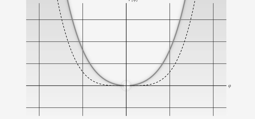
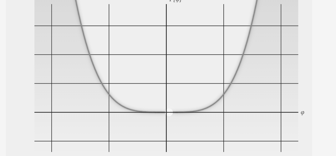
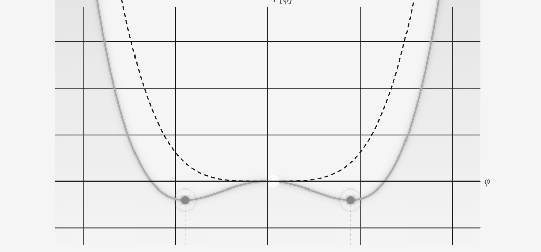
4.7. Summary of the threshold half

Not every tension imbalance produces a universe. This section derives a critical tension value, the modal threshold $\tau$ , below which the substrate remains abstract and unobservable, and above which it cannot remain that way. Think of water vapour: it can exist invisibly up to a certain temperature, but above that point it must condense. Below $\tau$ , the configuration has a single stable resting state with no geometry; above $\tau$ , that resting state becomes unstable and geometry must appear. The threshold is not assumed: it is calculated as the exact tension value at which the mathematical potential changes from single-welled to double-welled, and its existence is a structural necessity rather than a postulate.

The two postulates in play across this half are P2 (asymmetric vector tension, with $T(D)\neq 0$ in $V_{7}$ generically) and P3 (the $G_{2}$ -invariant Landau-Ginzburg modal potential on $V_{7}$ ); from them follow the existence and value of the modal threshold $\tau$ as the bifurcation point of $F[\psi,\varepsilon]$ and the vacuum manifold $\mathcal{V}\cong S^{6}\subset V_{7}$ for $\varepsilon>0$ . One point is worth disclosing explicitly: at the angular level the vacuum direction is not a spontaneous choice but is pinned by P2’s $\hat{\tau}$ , while at the discrete $Z_{2}$ level the symmetry breaking is genuinely spontaneous in the standard sense; these layered roles are made explicit in the “structural versus spontaneous asymmetry” paragraph. The modelling choices are the $G_{2}$ -invariant quartic functional form and the Bernoulli measure of § 2 as the configuration-space measure under which $F$ is varied.

4.8. The character of the threshold

What obtains at the modal threshold is unlike any physical process encountered in the instantiated world. It has no duration, no mechanism, no intermediate states, and no energy cost. It is not that it is very fast; temporal concepts simply do not apply to it. The precausal substrate is a nonspatiotemporal domain: there is no time in which a process could unfold, and no space across which it could propagate. What holds at the threshold is not a process but a modal reorganisation: a supra-threshold configuration is instantiated as geometry, where a sub-threshold one is not, and the two descriptions stand in this relation tenselessly.

Modal sublimation names this tenseless instantiation relation between the substrate description and the geometric description; it is not an event connecting two times. The substrate’s priority over geometry is logical and structural, not temporal: a supra-threshold configuration cannot remain uninstantiated by logical necessity (§12.8), and that logical priority, not a temporal one, is exactly what “precausal” means. Apparent processual language throughout this book, “crossing the threshold,” “the transition,” “the order parameter relaxes,” “the system settles”, is shorthand for that relation; no temporal process at the substrate level is implied.

The name sublimation is by analogy with the physical phenomenon in which a solid passes directly into a gaseous state, bypassing the liquid phase. In modal sublimation, every intermediate mode is bypassed because only two modes of being are available: uninstantiated existence within the precausal substrate, and instantiated existence as geometry. There is no intermediate mode that is partially spatial or partially causal.

Modal sublimation is characterised by four properties:

•

Nontemporal: no before or after, no duration, no sequence of states; the configuration is instantiated with time, not located within a pre-existing time
•

Nonmechanistic: no propagating influence, no force, no interaction
•

Nonenergetic: no conservation law, no energy input or output
•

Strictly modal: a change in the mode of being, not a change of state within an existing mode

Each of these four properties requires unpacking, because each contradicts a default assumption carried over from the instantiated world.

The nontemporal character is the most radical. In everyday physics, every process unfolds in time: there is a before and an after, a cause and an effect, a duration that can in principle be measured. Even processes described as instantaneous in non-relativistic mechanics, a collision, a decay, a measurement, are idealised limits of processes that have a finite, if arbitrarily small, duration. Modal sublimation is not a limit of this kind. It does not occur quickly; it does not occur in time at all. The configuration does not spend even an infinitesimal moment in transition. The reason is not dynamical but ontological: time is a structure of the instantiated domain, while instantiation is what constitutes that domain, not an event occurring within a prior time. To ask how long modal sublimation takes is to apply a concept to a context in which the concept has not yet been defined. This is not a failure of measurement precision; it is a logical impossibility of the same kind as asking what temperature a mathematical proof achieves. The configuration is not located within time; time is carried as a consequence of instantiation, not presupposed as a container in which a transition could unfold.

The nonmechanistic character follows directly from the nontemporal character. In the instantiated domain, every change of state is mediated by an interaction: a force, a field, a messenger particle, a propagating influence of some kind. These mediators all require spacetime in which to propagate and physical degrees of freedom to couple to. The precausal substrate has neither. No interaction can mediate the modal sublimation because interactions are structures of the domain that sublimation brings into being. There is no force that pushes a configuration across the threshold; the threshold is not a barrier that must be overcome but a logical boundary at which a particular mode of being ceases to be available. The transition is not driven by anything external. It is a logical consequence of the modal structure of the configuration itself, in the same way that the truth of a mathematical theorem is not caused by anything but follows necessarily from the axioms. This has a crucial implication: PST does not require a mechanism, an initial impetus, or a first cause. The demand for a mechanism is itself an instantiated-world concept, and applying it to the transition that precedes instantiation is a category error of the same kind as the causal question discussed in Chapter 5.

The nonenergetic character removes the last temptation to treat modal sublimation as a physical event in disguise. Energy is a conserved quantity defined within the instantiated domain: it requires a Hamiltonian, a time-translation symmetry via Noether’s theorem [21], and ultimately a spacetime manifold on which these structures can be defined. None of these are available in the precausal substrate. The relevant conservation statement in PST is not energetic but modal: it is the preservation of the asymmetric tension functional $T(C)$ across the threshold. The tension that characterises the precausal configuration is the same quantity that, after projection via $\Pi$ , appears as the stress-energy tensor $T_{\mu\nu}$ in the instantiated domain, as shown in Chapter 7. The Einstein field equations, on this reading, are not equations of motion governing a physical process; they are a conservation statement expressing that the structural content of the precausal configuration is faithfully preserved in the instantiated geometry. Nothing is created across the threshold; nothing is destroyed. The same structural content is expressed in a different modal register, the way that the same logical argument can be expressed in different formal languages without gaining or losing content.

The strictly modal character is the most philosophically precise formulation of what the other three properties imply. A change of state within an existing mode, a particle moving, a field oscillating, a temperature rising, leaves the mode of being intact while altering something within it. The ontological register is unchanged: the system is still a physical system in spacetime, governed by the same causal laws, measured in the same units. Modal sublimation changes the mode itself. The configuration does not acquire new properties within the precausal substrate; it changes the ontological register in which all its properties are expressed. Before sublimation, the configuration’s structural content exists as modal tension in a nonspatiotemporal domain. After sublimation, that same structural content exists as geometric curvature and matter-energy in a Lorentzian manifold. There is no moment at which the configuration is partially in each mode; the two modes stand in a strictly modal relation, not a temporal one, even though the phrasings “before” and “after” used here strictly apply only after time has come into being. This is the precise sense in which PST’s fundamental relation is irreducible to any physical process: physical processes are changes of state within the instantiated mode, while modal sublimation is the relation that constitutes the mode itself, not a happening within it.

The result of this transition is a geometry: a Lorentzian manifold $(M,g)$ that becomes the spacetime background for all subsequent physical processes. Geometry does not emerge within spacetime; it becomes spacetime in the act of sublimation.

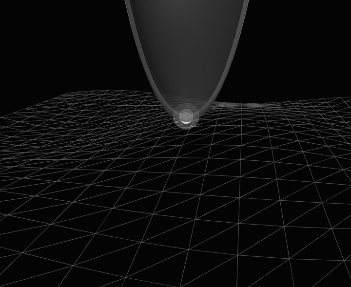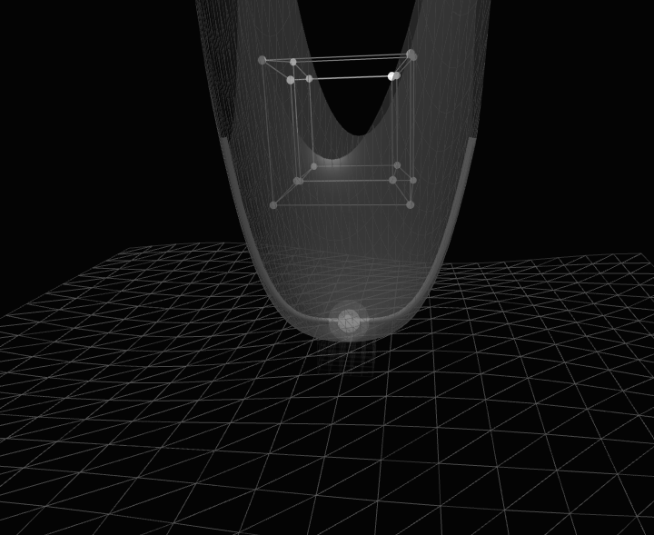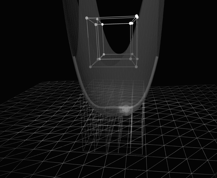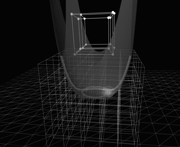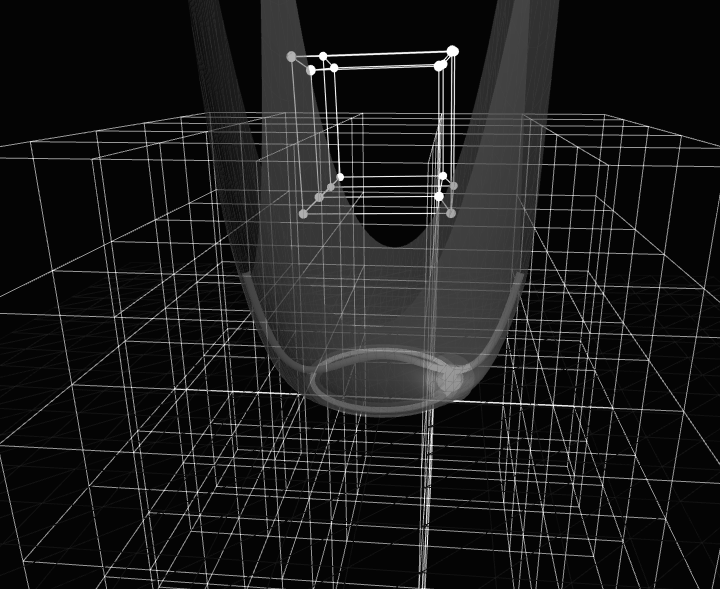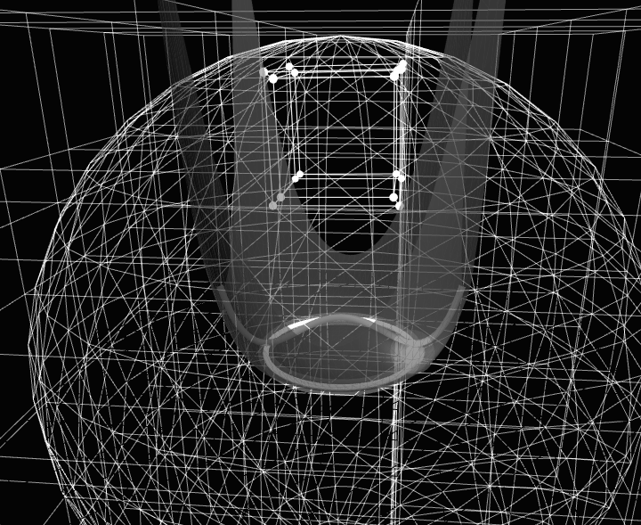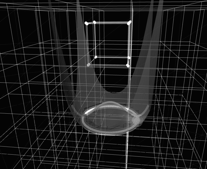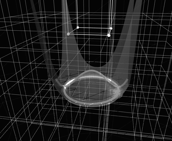4.9. Categorical formulation

The mathematical language suited to a transition between fundamentally different types of structure is category theory, specifically the theory of functors between categories [9]. Construct two categories as follows. The precausal category $\mathbf{S}$ has as objects all configurations $C\in\mathcal{C}$ with $T(C)\geq\tau$ , and as morphisms distinction preserving maps $f:C\rightarrow C^{\prime}$ . The geometric category $\mathbf{G}$ has as objects Lorentzian manifolds $(M,g)$ and as morphisms smooth maps preserving the causal structure.

Modal sublimation is the functor:

\Phi:\mathbf{S}\rightarrow\mathbf{G}

(28)

with four properties encoding the fundamental features of the transition:

1.

$\Phi$ exists at the categorical boundary; it is not a morphism within $\mathbf{S}$ or $\mathbf{G}$ , formalizing the nonmechanistic character of the transition
2.

$\Phi$ carries tension into geometry: the pairwise tensions fix the metric $g$ of the instantiated manifold via equation (29), and the tension projection $\Pi$ (equation (31)) supplies the stress-energy $T^{(\mathrm{iso})}_{\mu\nu}$ ; scalar curvature then follows from $g$ through the field equations of §7
3.

$\Phi$ is surjective: every Lorentzian manifold arises as the image of some precausal configuration
4.

$\Phi$ has no inverse: once a configuration is instantiated, the geometric domain has no access to the precausal substrate that produced it

4.10. Explicit construction of $\Phi$

The projection functor $\Phi$ inherits the post-sublimation directional structure of the substrate: it is constructed relative to the $\hat{\tau}$ -direction that modal sublimation locks (P2). The construction below produces a spacetime $M$ and a realisation $\rho$ together with an internal-factor identification along $\hat{\tau}$ ; the same construction at a different $\hat{\tau}^{\prime}\in S^{6}$ would produce a $G_{2}$ -rotated copy of the same $\Phi$ , with the rotation an unphysical relabelling. Once $\hat{\tau}$ is fixed by the substrate’s directional bias, $\Phi$ is determined up to the gauge freedom described below.

The functor is constructed in three steps.

Step 1, Geometric realization. The manifold $M$ and the map $\rho$ are not given independently before the construction; they are jointly determined by it.

A legitimate concern requires attention before the construction proceeds. The notation $\rho:D\rightarrow M$ appears to presuppose $M$ , a set of spacetime points, before the construction that is supposed to produce spacetime has been carried out. If spacetime points are already available as the target of $\rho$ , then the theory has not derived spacetime from the substrate; it has merely labeled pre-existing points with properties from $D$ . This would be a foundational circularity.

The resolution is that $M$ is not given prior to and independently of $\rho$ . The construction proceeds in the following order. First, note that any surjective function $\rho:D\twoheadrightarrow X$ , for any set $X$ , partitions $D$ into equivalence classes: $a\sim_{\rho}b$ if and only if $\rho(a)=\rho(b)$ . The equivalence classes $[a]_{\rho}=\{b\in D:\rho(b)=\rho(a)\}$ are the fibres of $\rho$ , and their collection $D/{\sim_{\rho}}$ is a quotient set that depends only on $D$ and the partition, not on any property of $X$ . A spacetime point is then defined to be a fibre of $\rho$ : it is an equivalence class of properties, not a pre-existing geometric entity. The manifold $M$ is the quotient set $D/{\sim_{\rho}}$ equipped with whatever additional structure (topology, differentiable structure, metric) the subsequent steps impose. The map $\rho$ is thus a quotient map, and $M$ is a derived set: it comes into existence as the image of $\rho$ , rather than being a container that $\rho$ maps $D$ into.

This construction has a philosophical precedent in Leibniz’s principle of the identity of indiscernibles: things that share all the same properties are the same thing. Here, the converse is operative, properties that are assigned to the same geometric locus by $\rho$ are identified, and the locus is nothing over and above that identification. A spacetime point has no content beyond the property-bundle it collects; it is not an additional ontological entity.

More concretely: $M$ is characterised as any smooth manifold of dimension $n$ whose topology and differential structure are consistent, a posteriori, with requiring that the metric constructed in Step 2 is well-defined and smooth. Among all candidate manifolds satisfying this consistency condition, the tension structure of $(D,\delta)$ further constrains which are admissible: a candidate $M$ is admissible if and only if there exists a partition of $D$ whose induced tension structure $T(\{[a],[b]\})=T(\{a,b\})$ reproduces the relational data already present in $(D,\delta)$ . This constraint, not an external stipulation, selects the spacetime topology and dimension.

Given a choice of admissible $M$ , define the realization map $\rho:D\rightarrow M$ as the quotient projection sending each property $a\in D$ to its equivalence class $\rho(a)=[a]_{\rho}\in M$ . The nonuniqueness of $\rho$ , the freedom to partition $D$ into fibres in multiple ways that are all consistent with the tension structure, is precisely the diffeomorphism invariance of General Relativity [1, 10]. It emerges here as a consequence of the nonuniqueness of geometric realization from the pre-geometric substrate, rather than as a separately imposed symmetry. There is no canonical labeling of spacetime points: this is not a deficiency of the theory but a structural result, matching the gauge freedom of GR.

Step 2, Tension-to-metric map. Introduce the null threshold $\tau_{\mathrm{null}}\in\mathbb{R}^{+}$ as the pairwise-tension companion of $\tau$ , determined jointly with $\tau$ rather than posited as an independent input. While $\tau$ is a condition on the global tension $T(C)$ , $\tau_{\mathrm{null}}$ is a condition on pairwise tensions $T(\{a,b\})$ : it is the value at which the two-property tension is null, i.e., at which $g=0$ by definition. The two thresholds operate at different levels. Their relationship reduces to the same open structural input as the rate-integral computation of §11.7: an explicit form of the global tension functional $T(C)$ as a functional of the pairwise tensions $T(\{a,b\})$ at the postulate level. Once the explicit functional is specified, $\tau$ is the critical value of $T(C)$ at which the modal potential loses its single-well stability (§4.1) and $\tau_{\mathrm{null}}$ is its pairwise restriction; the two are then determined jointly, not independently. The metric is then:

g_{\mu\nu}\!\left(\rho(a),\rho(b)\right)=\eta_{\mu\nu}\cdot\operatorname{sgn}% \!\left(\tau_{\mathrm{null}}-T(\{a,b\})\right)\cdot\left|T(\{a,b\})-\tau_{% \mathrm{null}}\right|^{1/2}

(29)

where $\eta_{\mu\nu}$ is a placeholder for the diagonal sign pattern $\mathrm{diag}(+1,-1,-1,-1)$ that the construction induces, not a presupposition of Minkowski geometry. Its appearance here is definitional: the signature theorem below shows that the sign pattern is fixed, downstream of the tension structure, by hyperbolic well-posedness of the Goldstone wave equation; $\eta_{\mu\nu}$ names that pattern, the mostly-minus signature $(+,-,-,-)$ used throughout (the Clifford convention $\gamma_{0}^{2}=+I$ , $\gamma_{i}^{2}=-I$ , giving the local Dirac algebra $\mathrm{Cl}(1,3)\cong M_{2}(\mathbb{H})$ , §8). This gives:

•

$T(\{a,b\})=\tau_{\mathrm{null}}\;\Rightarrow\;g=0$ : null separation
•

$T(\{a,b\})>\tau_{\mathrm{null}}\;\Rightarrow\;g<0$ : spacelike
•

$T(\{a,b\})<\tau_{\mathrm{null}}\;\Rightarrow\;g>0$ : timelike

The Lorentzian signature is forced as a theorem by hyperbolic well-posedness of the Goldstone wave equation (Computation 2, §13): the Cauchy problem for $\Box_{g}\theta=0$ admits a well-posed initial-value formulation and a conserved Noether current only for signature $(1,n-1)$ . The bifurcation of tension values around $\tau_{\mathrm{null}}$ remains the algebraic mechanism inside the LG variational structure; what Computation 2 shows is that the sign cut required for that bifurcation is not an independent axiom but a consequence of the well-posedness condition.

Two clarifications are necessary. First, equation (29) is strictly a pairwise assignment: it attaches a signed scalar to each pair of realised points, not a $(0,2)$ -tensor to a tangent space. The metric tensor field $g_{\mu\nu}(x)$ is recovered by the continuum limit: take $a$ and $b$ to be nearby properties such that $\rho(a)$ and $\rho(b)$ approach $x$ along a tangent vector $v^{\mu}$ ; then $g_{\mu\nu}(x)\,v^{\mu}v^{\nu}$ arises as the limit of equation (29) along the chord, analogous to recovering a Riemannian metric as the Hessian of a distance function. Second, the magnitude $\bigl{|}T(\{a,b\})-\tau_{\mathrm{null}}\bigr{|}^{1/2}$ is the minimal-regularity choice: a linear dependence would give a metric with a non-smooth gradient at the null cone, while the square root yields Hölder- $\tfrac{1}{2}$ behaviour there, the appropriate regularity class for a structure that degenerates at $T=\tau_{\mathrm{null}}$ and which ensures that equation (183) blows up precisely at the modal null threshold rather than at $T=0$ .

Step 3, Action on morphisms. For $f:C\rightarrow C^{\prime}$ in $\mathbf{S}$ , $\Phi(f):(M,g)\rightarrow(M^{\prime},g^{\prime})$ is the diffeomorphism induced by $f$ via $\rho$ . Distinction preserving maps in $\mathbf{S}$ correspond precisely to causal structure preserving maps in $\mathbf{G}$ , ensuring functoriality.

The projection operator. Define the tension projection operator $\Pi$ :

\Pi(T(C))(x)=\int_{\mathcal{C}}T(C^{\prime})\cdot K(x,C^{\prime})\,d\mu(C^{% \prime})

(30)

where $K(x,C^{\prime})=\delta(x-\rho(C^{\prime}))$ for local configurations. The role of $\Pi$ here is structurally analogous to the Dirac operator in Connes’ noncommutative geometry [48]: in both cases a single operator bridges an underlying non-spatial structure to the instantiated domain (the metric itself is supplied by $\Phi/\rho$ , not by $\Pi$ ). The stress-energy tensor at $x\in M$ in the isotropic, homogeneous case is:

T^{(\mathrm{iso})}_{\mu\nu}(x)=\Pi(T(C))(x)\cdot g_{\mu\nu}(x)

(31)

This isotropic scalar form $T^{(\mathrm{iso})}_{\mu\nu}=\Pi(T(C))\,g_{\mu\nu}$ gives a stress-energy tensor proportional to the metric, which is the correct structure for a cosmological constant ( $T_{\mu\nu}=\Lambda g_{\mu\nu}$ ) but not for general matter distributions. Pressurised matter, radiation, and anisotropic fields all have $T_{\mu\nu}\neq\lambda g_{\mu\nu}$ for any scalar $\lambda$ . The general form requires $\Pi$ to be a tensor-valued projection $T_{\mu\nu}(x)=\Pi_{\mu\nu}(T(C))(x)$ , whose components encode the directional distribution of tension in the precausal configuration. The scalar form is the leading-order approximation valid for isotropic configurations; the full tensor generalisation is an open problem. The noninvertibility of $\Phi$ is immediate: $\rho$ discards the internal structure of $D$ that does not affect pairwise tensions. Geometry encodes the projection of $T$ through $\Pi$ but not the full precausal configuration that generated it, just as a shadow records an object’s outline but not its internal structure.

4.11. Uniqueness of $\Phi$ and the origin of diffeomorphism invariance

The construction proceeds via an explicit choice of realization map $\rho:D\rightarrow M$ , which is not determined by the precausal structure alone. This raises the question of how strongly the output functor $\Phi$ depends on the choice of $\rho$ , and what that dependence implies for the physical content of the theory. The answer is a uniqueness theorem: $\Phi$ is unique up to diffeomorphism, and the ambiguity in $\Phi$ is completely and exactly characterised by diffeomorphism invariance, with no residual freedom beyond it.

The proof follows directly from the construction. Given $\rho$ , the metric $g_{\mu\nu}$ at every pair of points is fully determined by equation (29): there are no further choices once the realization map is fixed. Now suppose $\rho^{\prime}=f\circ\rho$ for some smooth bijection $f:M\rightarrow M^{\prime}$ . The tension values $T(\{a,b\})$ depend only on $a,b\in D$ , not on their images under $\rho$ , so they are unchanged by the substitution. Therefore the metric computed at $(\rho^{\prime}(a),\rho^{\prime}(b))$ via equation (29) satisfies $g^{\prime}(\rho^{\prime}(a),\rho^{\prime}(b))=g(\rho(a),\rho(b))$ , which is exactly the condition that $(M^{\prime},g^{\prime})$ is the pushforward of $(M,g)$ along $f$ . Any two choices of $\rho$ therefore produce Lorentzian manifolds that are diffeomorphic to one another, together with a corresponding natural isomorphism between the two functors they define. $\Phi$ is unique up to this natural isomorphism, which at the level of manifolds is a diffeomorphism.

What the uniqueness theorem leaves open is not a further gauge choice but which substrate configuration is instantiated: the realization map $\rho$ is fixed up to diffeomorphism once the configuration is given, but the theory must still say which configuration sublimation realises. P3 supplies this through maximum entropy: modal sublimation instantiates the $\mu$ -typical (maximum-entropy) configuration, not a $\mu$ -exceptional one. The permutation symmetry of the substrate measure already forces equidistribution in measure; maximum-entropy sublimation strengthens this to the realised configuration itself, so its emergence cloud $\rho_{n}$ is metric-covariantly equidistributed at the closure rate $\eta_{K,R}<d_{0}^{2}/4$ . This is exactly condition A3 of the Mosco limit (§7.7); it therefore holds as a consequence of P3, and the Mosco convergence to $M=\mathbb{R}\times S^{3}$ is unconditional. The selection is a typicality principle internal to P3, the analogue of maximum-entropy or generic-initial-data selection elsewhere in physics: it adds no fourth postulate and derives no rate from more primitive structure, but it locates the equidistribution where it belongs, in the dynamics of instantiation.

The physical significance of this result is that diffeomorphism invariance in General Relativity is not an additional symmetry requirement that must be imposed upon the theory by hand. It is the complete characterisation of the non-uniqueness of $\Phi$ : the relabelling freedom in choosing $\rho$ survives into the instantiated manifold as coordinate freedom, and coordinate freedom is diffeomorphism invariance. There is no finer ambiguity and no coarser one; the two are identical. The natural question of whether $\Phi$ is unique and what physical symmetries characterise its ambiguities is therefore answered here: $\Phi$ is unique up to diffeomorphism, its ambiguity is completely characterised, and the physical symmetry corresponding to that ambiguity is diffeomorphism invariance.

A note on the metric signature. The argument in Step 2 assigned the Minkowski signature $(+,-,-,-)$ through equation (29), by bifurcating pairwise tensions about a null threshold $\tau_{\mathrm{null}}$ that separates spacelike from timelike separations. This determines the signature given $\tau_{\mathrm{null}}$ : once a sign cut is supplied, $T>\tau_{\mathrm{null}}$ is spacelike and $T<\tau_{\mathrm{null}}$ is timelike, by construction. It does not determine that exactly one direction lies below $\tau_{\mathrm{null}}$ , spectral asymmetry of the tension spectrum about a threshold (the standard form of which is $T(C)\neq T(\bar{C})$ , complement-asymmetry) is consistent with zero, one, or several eigenvalues lying below any given cut, so it does not by itself fix the count of timelike directions. Equivalently: in the multidimensional-scaling reframing of the realisation map (§13), any $S_{D}$ -invariant Gram construction over real features is positive-semidefinite by elementary linear algebra, so the negative eigenvalue required for one timelike direction cannot arise from $S_{D}$ -symmetry alone; it must be supplied by an indefinite bilinear form beyond the Gram construction. The Lorentzian signature $(+,-,-,-)$ is fixed as a theorem via Computation 2 of §13: hyperbolic well-posedness of the Goldstone wave equation forces $(p,q)=(1,n-1)$ , and the $\mathrm{U}(1)$ Noether-current conservation that produces the angular-momentum identification requires this same Lorentzian signature. The macroscopic dimension $n=4$ that combines with the signature to give the four-dimensional Lorentzian spacetime $M=\mathbb{R}\times S^{3}$ follows from KO additivity given the verified spectral-triple structure (§1.5): the substrate’s parity-selected KO-6 (Computation 3) and the product’s KO-2 mod 8 (Connes Lorentzian value) together force $M$ at KO-dimension four. PST is then the theory that derives everything downstream from $(D,\delta)$ + LG + the realisation map $\rho$ , with both signature and macroscopic dimension outputs rather than inputs.

4.12. Lorentzian signature from Goldstone hyperbolic well-posedness

This subsection makes self-contained the result that Lorentzian signature follows from hyperbolic well-posedness of the Goldstone wave equation (Computation 2): we state the PDE, the function spaces, the energy estimate, and show why one timelike direction (signature $(p,q)=(1,n-1)$ ) is the unique signature compatible with a well-posed Cauchy problem on the projected spacetime $\mathbb{R}\times S^{3}$ .

The logical order forestalls any apparent circularity. The manifold $M=\mathbb{R}\times S^{3}$ and its differentiable structure emerge first, as the Mosco limit of the Boolean Dirichlet form (§7.6), carrying a topology but as yet no metric signature; the signature is then fixed downstream as the unique one for which the Goldstone wave equation on that already-emergent manifold admits a well-posed Cauchy problem. Hyperbolicity does not presuppose a metric, it selects among the candidate signatures available on a manifold that exists prior to any of them.

The PDE. After modal sublimation has selected the vacuum manifold $\mathcal{V}\cong S^{6}\subset V_{7}$ (§1.7, P3), the Goldstone phase $\theta$ along the broken direction satisfies, at the quadratic order of the LG functional, the second-order PDE

g^{\mu\nu}\,\partial_{\mu}\partial_{\nu}\,\theta(x)\;=\;0,\qquad x\in M,\;\;% \mu,\nu=0,1,\ldots,n-1,

(32)

where $g^{\mu\nu}$ is the (Wick-rotation-undetermined) [161] signature- $(p,q)$ metric on $M=\mathbb{R}\times S^{3}$ obtained as the projection of the LG kinetic term to emergent spacetime. The order parameter contributes $r_{0}^{2}|\nabla\theta|^{2}$ to the LG free energy, which under $\nabla\to g^{\mu\nu}\partial_{\mu}\otimes\partial_{\nu}$ becomes the wave operator.

Cauchy problem and function spaces. The Cauchy problem for equation (32) on the time slice $\Sigma_{0}=\{0\}\times S^{3}$ asks: given initial data $(\theta_{0},\theta_{1})\in H^{1}(S^{3})\times L^{2}(S^{3})$ , does there exist a unique solution $\theta\in C(\mathbb{R};H^{1}(S^{3}))\cap C^{1}(\mathbb{R};L^{2}(S^{3}))$ with $\theta|_{\Sigma_{0}}=\theta_{0}$ , $\partial_{t}\theta|_{\Sigma_{0}}=\theta_{1}$ ?

For the Cauchy problem to be well-posed in the Hadamard sense [110] (existence, uniqueness, and continuous dependence on initial data) the principal symbol $g^{\mu\nu}\xi_{\mu}\xi_{\nu}$ of equation (32) must be strictly hyperbolic with respect to the splitting $\Sigma_{0}$ , i.e. the polynomial

g^{00}\omega^{2}\;+\;2g^{0i}\omega\xi_{i}\;+\;g^{ij}\xi_{i}\xi_{j}\;=\;0

(33)

must have exactly two real roots $\omega=\omega_{\pm}(\xi)$ for every nonzero spatial covector $\xi\in T^{*}\Sigma_{0}$ [113, 114, 99]. Strict hyperbolicity forces the metric to have one timelike direction (transverse to $\Sigma_{0}$ ) and $n-1$ spacelike directions. Equivalently, signature $(p,q)=(1,n-1)$ (or its sign-reversal $(n-1,1)$ , the same content).

Energy estimate. Given strict hyperbolicity, multiplying equation (32) by $\partial_{t}\theta$ and integrating over $\Sigma_{t}$ yields the standard wave energy

E(t)\;=\;\tfrac{1}{2}\int_{\Sigma_{t}}\bigl{(}\,(\partial_{t}\theta)^{2}\;+\;g% ^{ij}\partial_{i}\theta\,\partial_{j}\theta\,\bigr{)}\sqrt{g_{S^{3}}}\,dx

(34)

which is conserved: $E(t)=E(0)$ for all $t\in\mathbb{R}$ . Energy conservation immediately gives existence (via the standard semigroup construction [99]), uniqueness (the zero-data Cauchy problem has zero energy and hence zero solution by Gronwall), and continuous dependence (initial-data perturbations propagate at finite speed bounded by $\max|g^{ij}/g^{00}|^{1/2}$ along light cones). This is the standard Sobolev-space well-posedness theory for the wave equation [113, 114].

What fails in other signatures. Three alternatives must be considered and ruled out:

1.

Euclidean $(p,q)=(0,n)$ . All directions are spacelike; the principal symbol $g^{\mu\nu}\xi_{\mu}\xi_{\nu}$ is positive-definite. Equation (32) becomes elliptic (Laplace) rather than hyperbolic. The Cauchy problem for an elliptic equation is famously ill-posed (Hadamard’s classical example [110]): small perturbations in the data give exponentially growing perturbations in the solution, so no continuous-dependence map exists. Modal sublimation produces a domain that admits time evolution, not an elliptic boundary-value problem; Euclidean signature is therefore incompatible with the Cauchy-problem structure of modal sublimation.
2.

Ultra-hyperbolic $(p,q)$ with $p\geq 2$ , $q\geq 2$ . Two or more timelike directions. The principal symbol has signature $(p,q)$ as a quadratic form, but the Cauchy problem on the codimension- $p$ “time” submanifold has multiple time derivatives in the data, and strict hyperbolicity in the sense above fails: the polynomial in $\omega$ has either no real roots (for some $\xi$ ) or more than two. The Cauchy problem is ill-posed in the Hadamard sense; existence fails for generic smooth data [111, 112].
3.

$(p,q)=(n,0)$ (anti-Lorentzian). All directions timelike, no spatial direction. Equation (32) has no propagation direction; the projection has no instantiated geometry to speak of. Excluded as a degenerate case.

Conclusion. The unique signature compatible with a well-posed Cauchy problem for the Goldstone wave equation on the Mosco-limit spacetime $M=\mathbb{R}\times S^{3}$ is $(p,q)=(1,n-1)$ . Combined with the $n=4$ fix from the minimal KO-split (§1.5), this gives $(p,q)=(1,3)$ , i.e. signature $(+,-,-,-)$ . Lorentzian signature is therefore a theorem of modal sublimation rather than an additional postulate: the directionality of the threshold crossing selects time, hyperbolic well-posedness selects the number of spatial directions, and Computation 2 verifies the explicit energy-estimate construction numerically on representative finite models.

The above is a structural derivation using standard PDE theory [113, 114, 99]; the energy estimate is rigorous and the alternative-signature arguments are sketched at standard textbook level rather than fully worked. A fully rigorous treatment with detailed Sobolev-space analysis is straightforward but would expand the appendix substantially; the structural conclusion does not depend on which level of analytic detail one prefers. Computation 2 supplies the numerical verification of energy conservation on a finite-mode truncation of $S^{3}$ .

4.13. Summary

Modal sublimation is the moment the threshold is crossed, not a moment in time, but a logical transition. When a configuration’s tension exceeds $\tau$ , it cannot remain in its abstract precausal state; it is compelled, by the same kind of necessity that makes a mathematical theorem true, to become concrete. The result is a four-dimensional spacetime with the Lorentzian signature that physics recognises. This section constructs the map from the precausal domain to the geometric domain, shows it is unique, and proves that the coordinate-freedom of General Relativity (diffeomorphism invariance) is a consequence of that uniqueness rather than a separate postulate.

Concretely, the modal-sublimation functor $\Phi:\mathcal{S}\to\mathcal{G}$ is constructed explicitly in three steps. Its central derived result (Computation 2) is that hyperbolic well-posedness of the Goldstone wave equation along $\hat{\tau}$ forces the Lorentzian signature $(+,-,-,-)$ ; the energy-estimate and PDE details are sketched here, with an expanded self-contained derivation left to future work, and the existence of the sign cut at $\tau_{\mathrm{null}}$ , where hyperbolicity flips, follows from that well-posedness requirement rather than being posited, while its value is determined jointly with $\tau$ through the explicit form of $T(C)$ (§11.7). Diffeomorphism invariance is likewise derived, from the non-uniqueness of the realisation map $\rho$ . The passage $\mathcal{S}\to M=\mathbb{R}\times S^{3}$ is an unconditional theorem (under P1–P3) resting on Mosco convergence of the Boolean Dirichlet form to the Laplace-Beltrami form on $M$ : the argument is structural, stated explicitly in §7.7 with seven assumptions A1–A7, and the equicoercivity A7 is an unconditional theorem of §7.7, combining its equidistribution condition A3 (a uniform-rate hypothesis (R) on $H^{1}$ -bounded compactly-supported test functions), supplied by P3’s maximum-entropy sublimation, with a standard Poincaré inequality; A3 is corroborated for the i.i.d. surrogate (Computation 70), which confirms the rate P3 supplies for the emergence-determined cloud. The one extremal modelling choice is the minimal KO-split $4+6=10$ given the KO- $6$ substrate (§1.5), which fixes $n=4$ .

5. Coinstantiation of Spacetime and Causality

5.1. Causality as coinstantiated structure

The previous section established that modal sublimation is a nontemporal, nonmechanistic transition: the functor $\Phi:\mathbf{S}\rightarrow\mathbf{G}$ maps a precausal configuration directly into a Lorentzian manifold without passing through any intermediate state and without requiring a prior temporal structure in which the transition could unfold. A consequence of this that deserves its own careful treatment is the status of causality itself. Causality is not, in PST, a background structure that was already present when the universe formed and that can then be applied to the event of its formation. Causality is coinstantiated with geometry: it arises at the same moment as the Lorentzian manifold that carries it, because it is constitutively defined in terms of that manifold. There is no moment, however brief or abstract, at which a causal relation exists but spacetime does not. The two are ontologically inseparable.

This point carries weight precisely because it is not obvious. Much of the philosophical and cosmological literature treats causality as prior to or more fundamental than spacetime. In the Kantian tradition, causality is a category of the understanding applied to experience, logically prior to any empirical fact about the world [34]. In causal set theory, the discrete partial order is the primary structure from which the continuum metric is to be recovered [4, 35]. In quantum gravity approaches that proceed via sum over histories, the causal structure of each history is taken as given, and the amplitude is computed over those histories [36]. Even in ordinary language, the question “what caused $X$ ?” is considered answerable in principle for any event $X$ , the presumption being that every event has a cause and that the causal relation is always available to be invoked.

PST disagrees at the foundational level. The precausal substrate, as defined in Chapter 2, does not possess a causal order. It possesses property differentiation and the tension functional. These are not impoverished substitutes for causality; they are genuinely different kinds of structure. The distinction relation $\delta$ is symmetric and irreflexive: it registers that two properties differ from each other without specifying which is prior to the other or whether either depends on the other. The tension functional $T$ assigns a magnitude to a configuration without implying that one configuration succeeds or precedes another. Neither $\delta$ nor $T$ contains the ingredients from which a temporal order could be constructed. A temporal order requires at minimum an asymmetric, transitive relation on a set of events. The precausal substrate has none. Causality is not absent from the substrate in the way that a feature might be absent from a description that was meant to include it; it is absent from the substrate in the sense that the substrate belongs to a logical type to which causal relations do not apply.

5.2. Mathematical formulation of coinstantiation

Let $(M,g)=\Phi(C)$ be the Lorentzian manifold produced by modal sublimation of a configuration $C\in\mathbf{S}$ . The causal structure on $(M,g)$ is the partial order $\leq$ defined pointwise by the lightcone structure of $g$ :

p\leq q\;\iff\;q\in J^{+}(p,g)

(35)

where $J^{+}(p,g)$ is the causal future of $p$ under the metric $g$ :

	$\displaystyle J^{+}(p,g)=\{\,q\in M\;\mid$	$\displaystyle\exists\text{ future-directed causal curve }\gamma:[0,1]% \rightarrow M,$		(36)
		$\displaystyle\gamma(0)=p,\;\gamma(1)=q\,\}$		(36)

A curve is causal under $g$ if and only if its tangent vector $\dot{\gamma}$ is everywhere non-spacelike, that is $g(\dot{\gamma},\dot{\gamma})\geq 0$ at every point. This definition depends on $g$ in an essential way: the notion of a causal curve, and hence of causal precedence, is meaningless without a metric. Change the metric and the causal structure changes with it; remove the metric and the causal structure does not become unspecified but ceases to exist as a category of object.

The partial order $\leq$ in equation (35) has no pre-image in the precausal category $\mathbf{S}$ . Formally, there is no morphism or relation in $\mathbf{S}$ that maps to $\leq$ under $\Phi$ , because the objects of $\mathbf{S}$ are configurations equipped only with $\delta$ and $T$ . This is not a deficiency of the model; it is a structural theorem: the functor $\Phi$ is not surjective on structure but on objects. It produces a manifold but does not carry into that manifold a pre-existing causal order; the causal order is generated anew by the Lorentzian signature of the metric produced by equation (29). Therefore the following holds:

\text{causality}\;=\;f(g)\;=\;f(\Phi(C))

(37)

Causality is a derived relation, defined in terms of the metric, which is itself defined in terms of the precausal tension structure via $\Phi$ . It is not an independent primitive.

5.3. The direction of time as a structural consequence

The Lorentzian signature of the metric $(+,-,-,-)$ introduces an asymmetry that has no parallel in a purely Riemannian geometry. In a Riemannian manifold, all directions from a point are spacelike and the notion of a preferred future does not arise. In a Lorentzian manifold, the lightcone at each point divides the tangent space into two timelike halves, one conventionally designated as the future and the other as the past, and a continuous causal vector field on $M$ selects one half globally, providing a time orientation [37, 38].

In PST this asymmetry is not imposed as an additional datum. It is inherited from the asymmetry of the precausal substrate. Asymmetric tension, by definition, is a non-symmetric functional: $T(\bar{C})\neq-T(C)$ generically, where $\bar{C}$ is the complement of $C$ in $D$ . Across the functor $\Phi$ this asymmetry survives as the time orientation: the Lorentzian signature itself is fixed by hyperbolic well-posedness of the Goldstone wave equation (Computation 2), and the preferred time direction of the manifold reflects the substrate’s globally fixed modal-sublimation direction $\hat{\tau}\in V_{7}$ , locked at threshold crossing by P3. The thermodynamic arrow of time, the cosmological arrow of time, and the distinction between retarded and advanced solutions in electrodynamics are all grounded in this single asymmetry inherited from the substrate.

A technical caveat is required. The complement-asymmetry $T(\bar{C})\neq-T(C)$ (10) is a configuration-level condition; a global time orientation on $M$ requires a continuous nowhere-vanishing timelike vector field on the entire manifold. By Geroch’s theorem [37], a Lorentzian manifold is time-orientable if and only if such a field exists, which is a global topological condition not automatic from local asymmetry. In PST the global character of the precausal configuration $C$ provides the resource: the globally fixed modal-sublimation direction $\hat{\tau}\in V_{7}$ (the preferred direction identified in Chapter 4, fixed at threshold crossing by P3) gives a precausal structure that $\Phi$ maps to a candidate timelike field on $M$ .

The continuity and nowhere-vanishing of this field follow from three structural ingredients: (i) the modal-sublimation direction $\hat{\tau}\in V_{7}$ is fixed globally at threshold crossing (§1.7, P3), so it is a single non-vanishing element of $V_{7}$ rather than a configuration-dependent choice; (ii) the substrate-to-spacetime projection $\rho$ underlying $\Phi$ is permutation-equivariant under the substrate’s $S_{D}$ symmetry, by the same permutation-invariance argument (which forces the equidistribution assumption A2 of §7.7) that drives the cosmological-principle theorem (§11.5, “Theorem (Cosmological Principle)”); (iii) the Mosco-convergence framework of §7.7 delivers $\rho$ in the strong-resolvent topology, which preserves continuity of the projected direction. Combining (i)–(iii): $\hat{\tau}$ is mapped by $\Phi$ to a globally non-vanishing continuous timelike direction on $M=\mathbb{R}\times S^{3}$ ; specifically $\Phi(\hat{\tau})=\partial/\partial t$ along the $\mathbb{R}$ factor. Geroch time-orientability is therefore a structural consequence of the modal threshold (P3) plus the substrate permutation invariance plus the Mosco convergence, rather than an additional assumption.

5.4. The causal order and the degenerate vacuum

A further consequence of coinstantiation concerns the vacuum manifold. As established in Chapter 4, the post-threshold vacuum is the $V_{7}$ -vacuum sphere $\mathcal{V}\cong S^{6}$ . For the U(1) Goldstone-phase and angular-momentum analysis below, the relevant substructure is the 2-plane slice fixed by $\hat{\tau}$ and any perpendicular unit direction $\hat{\eta}\perp\hat{\tau}$ : the projected ring $\mathcal{V}_{\hat{\eta}}\cong S^{1}$ . Henceforth in this book, statements involving “ $\mathcal{V}\cong S^{1}$ ” refer to this projection, the U(1)-relevant slice of the full $S^{6}$ vacuum manifold (P3); the perpendicular five additional directions on $S^{6}$ carry the gauge-theoretic content (§8.15). Motion along $\mathcal{V}$ is the only stable state the vacuum admits. In the instantiated geometry, this motion projects under $\Pi$ into persistent non-vanishing stress-energy, which in turn sustains curvature. Crucially, the causal order $\leq$ treats this motion as part of the background structure: the lightcone structure generated by the projected metric encodes the vacuum motion as a baseline curvature rather than as a deviation from flatness. This is why the structural argument holds that orbital motion at all scales does not require an initial condition that specifies it separately: it is a candidate for the ground state of the causal structure. The explicit $\Pi$ -mapping connecting this Noether charge to the observed orbital angular momentum of massive bodies is computed in §7.21.

5.5. Category error and the dissolution of first-cause questions

With coinstantiation established, PST is in a position to address what is perhaps the most persistent question in the philosophy of cosmology: what caused the universe to come into being? The question appears legitimate. It has the grammatical form of a causal question, it points to a definite event (the coming-into-being of the universe), and it invites an answer of the form “ $X$ caused the universe”.

The question is not, however, answerable. It is not unanswerable in the sense that the answer is hidden or that the evidence has been destroyed; it is unanswerable because it commits a category error, applying a relation to an entity that belongs to a logical type to which the relation does not apply [39, 40]. To ask what caused the universe is to presuppose that the causal relation exists and is applicable to the event of the universe’s formation. But the causal relation, as shown above, is coinstantiated with the universe: it comes into being with the very event whose cause is being sought. A relation cannot serve as the explanation for the event that constitutes its own first instantiation.

The parallel with simpler category errors is instructive. “What is north of the North Pole?” presupposes that the directional relation north-of is defined at the North Pole, but the relation is defined only within the coordinate system that has the North Pole as its boundary. “What was there before the Big Bang?” presupposes that the relation earlier-than is defined at the Big Bang, but that relation depends on the spacetime whose earliest moment is the Big Bang. “What caused the universe?” presupposes that the causal relation is defined for the event of universal instantiation, but that relation depends on the very spacetime that is being instantiated. In each case the error is structural: the question applies a relation in a domain where that relation does not exist.

The dissolution of the category error is not a retreat. PST does not avoid the question by refusing to engage; it dissolves it by exhibiting the precise logical structure that makes it malformed. This dissolution is, moreover, constructive: in place of the unanswerable question, PST offers the answerable one. Why does the universe exist at all? Because the precausal substrate possesses property differentiation, and property differentiation entails asymmetric tension, and once tension exceeds the modal threshold, modal sublimation to instantiated geometry is logically necessary, not contingently triggered. The question Leibniz posed, “why is there something rather than nothing?” [41], receives not an arbitrary answer but a principled one: because the logical possibility of property differentiation is irreducible, and a substrate bearing irreducible property differentiation cannot remain uninstantiated once the threshold condition is satisfied. Existence is not a brute fact; it is the necessary expression of a logically unavoidable modal imbalance.

5.6. Contrast with competing approaches

Several approaches in the literature address the question of cosmological origins in ways that are instructive to compare with PST.

The Hartle-Hawking no-boundary proposal [36] avoids a boundary in time by making the metric Euclidean in the deep past, eliminating the initial singularity by changing the signature. This is technically elegant but it does not dissolve the category error: the sum over geometries is still computed within a pre-existing mathematical framework equipped with a notion of quantum amplitude, and the question of why that framework is instantiated rather than another is not addressed. The no-boundary proposal also treats causality as part of the background formalism rather than as a derived structure.

Vilenkin’s tunneling proposal [42] posits a quantum tunneling event from nothing. But “nothing” in this context is not the absence of structure; it is a specific quantum gravitational state with a precisely defined wave function. The transition from that state presupposes both quantum mechanics and the causal structure within which the transition is defined. The proposal is internally consistent but does not escape the regress: it pushes the question back to the prior state and the framework defining the transition.

Causal set theory [4] makes the causal partial order primitive and attempts to derive the continuum from it. This is in some respects the inverse of PST: where causal set theory starts with $\leq$ and tries to recover $g$ , PST derives both $g$ and $\leq$ from $\Phi$ . Causal set theory faces the question of what determines the particular causal set that becomes this universe, a question it answers by probabilistic sampling over a measure on causal sets. PST does not face this question in the same form: the particular geometry that arises is determined by the tension configuration $C$ , which is itself subject to the modal potential.

The position of PST is that all approaches that take causality as a starting point, whether as a background relation, a quantum mechanical framework, or a primitive partial order, are working within the instantiated domain and can at best describe the structure of what has been instantiated. The question of why anything is instantiated at all requires a theory that can speak from outside the instantiated domain. The precausal substrate, and the functor $\Phi$ through which it gives rise to geometry, is that theory.

5.7. Summary

Spacetime and the causal order (the fact that causes precede effects) do not arise one after the other. They are two aspects of a single transition and cannot exist independently of each other. This has a profound consequence: there is no “before” the universe, because time itself is part of what the transition produces. Asking what caused the universe is a category error, like asking what is north of the North Pole. The Big Bang is not a beginning at a point in time; it is what the transition looks like from inside the geometry it creates.

Nothing new is postulated in this chapter: causality co-emerges with geometry through the same modal-sublimation step, with no separate causal postulate added, and the arrow of time follows as a structural consequence of P2’s asymmetric tension direction $\hat{\tau}$ . The causal order itself is interpreted as the partial order on instantiated events induced by $\Phi$ , an interpretation consistent with the standard relativistic causal structure on $M$ .

6. The Emergence Chain

6.1. Overview and the eight-step summary table

The preceding four sections have built the foundations of PST step by step: from the single primitive of property differentiation, through asymmetric tension and the modal threshold, to modal sublimation and the coinstantiation of geometry and causality. This section draws those steps together into a single, unified chain of logical entailment and examines what that chain is, what kind of necessity binds each step to the next, what distinguishes it from competing accounts of emergence in physics, and what it means for the chain to be complete.

The table below summarises the eight steps that constitute the chain. Each entry names the emergent concept, gives the mathematical object that represents it, and implies a link to its predecessor. The prose that follows unpacks each link in turn.

Step	Concept	Mathematical object
1	Property differentiation	$(D,\delta)$ , a set with a symmetric, irreflexive distinction relation
2	Asymmetric tension	$T:\mathcal{C}\rightarrow\mathbb{R}^{+}$ , $T(C)\neq T(\bar{C})$ for all $C$
3	Modal threshold	Bifurcation point $\tau$ of $\mathcal{F}(\psi,C)$ , eq. (27)
4	Modal sublimation	Functor $\Phi:\mathbf{S}\rightarrow\mathbf{G}$ , constructed via $\rho$ and eq. (29)
5	Geometry as spacetime	Lorentzian manifold $(M,g)$ with signature supplied by $\tau_{\mathrm{null}}$
6	Causality	Partial order $\leq$ on $M$ via $J^{+}(p,g)$ ; no pre-image in $\mathbf{S}$
7	Energy, matter, fields	$T_{\mu\nu}=\Pi(T(C))\,g_{\mu\nu}$ ; $G_{\mu\nu}=8\pi G\cdot\Pi(T(C))\,g_{\mu\nu}$ ; bosonic field sector; fermionic content with structural spin-statistics from the CAR algebra on the Boolean distinction primitive (Chapter 8)
8	Angular momentum	Noether charge $L=2r_{0}^{2}\,\dot{\theta}$ of the $\mathrm{U}(1)$ symmetry of the 2-plane projection $\mathcal{V}_{\hat{\eta}}\cong S^{1}$ of the $V_{7}$ -vacuum sphere $\mathcal{V}\cong S^{6}$

6.2. The character of the chain

The first thing to establish is what kind of chain this is. It is not a causal chain. The steps do not follow each other in time; they are not events that happen sequentially in a universe that already exists. It is not an evolutionary chain in the sense used in cosmology, where one physical state develops into another under the action of laws that are themselves already given. The chain is a chain of logical entailment: each concept is not merely correlated with its successor but is the necessary and sufficient condition for it. Given step $n$ , step $n+1$ is not optional; it is logically unavoidable. Remove any link and the entire structure downstream collapses.

This is a stronger claim than is usually made in emergence theories. In most accounts, emergence is a relation between levels of description: a higher-level description emerges from a lower-level one when the higher-level regularities can, in principle, be derived from the lower-level equations. The chain has a direction but not a necessity. In PST the chain has both. The direction runs from the logically irreducible toward the structurally complex, and at every step the direction is the only one available. The question “why does tension arise from differentiation?” does not have an empirical answer, the sort of answer one would give by pointing to a law of nature or a measured constant. It has a logical answer: any configuration of two or more distinct properties contains non-identity internal relations, and those relations cannot collectively neutralise. Tension is not observed to follow from differentiation; it is entailed by it, together with the complement-asymmetry condition.

A precise statement of what the chain entails requires distinguishing two levels. At the structural level, the steps are necessary given the primitive and the structural commitments of PST: tension follows from distinctness together with the complement-asymmetry condition; the threshold follows from the existence of tension together with the commitment to a bifurcation structure; modal sublimation follows from the threshold by the instability argument; spacetime and causality coinstantiate via the functor $\Phi$ . At the architectural level, the specific mathematical objects representing each step, the Landau-Ginzburg functional, the gradient flow, the canonical measure, are the minimal motivated choices consistent with the structural requirements; they are not strictly entailed by $(D,\delta)$ alone, as the epistemological caveat of Chapter 2 makes explicit. Steps 3 through 8 are necessary given the structural encoding, which is itself logically motivated rather than derived. The chain is closed at the structural level; it is architecturally motivated at the representational level. This two-tier character is not a weakness; it identifies precisely where the foundational programme remains open and where future derivations could replace motivated choices with strict entailments.

6.3. Step 1 to Step 2: from differentiation to tension

Property differentiation is the capacity for distinctions to exist: the set $D$ equipped with the distinction relation $\delta$ , symmetric and irreflexive, requiring no loci, relata, or temporal structure. This is the single primitive from which the entire theory is built. Its logical irreducibility was established in Chapter 2: any attempt to explain why distinctions can exist already presupposes a context in which two things differ from each other, committing a circularity. The primitive cannot be grounded further without circularity; it can only be identified.

Asymmetric tension follows from differentiation together with the complement-asymmetry condition. A configuration $C\subset D$ drawn from a set of distinct properties admits internal non-identity relations. Since $\delta$ is symmetric, $\delta(a,b)$ and $\delta(b,a)$ hold simultaneously; these relations carry no preferred direction. The asymmetry in asymmetric tension is not directional but complementary: the structural condition that no configuration and its complement carry equal tension, $T(C)\neq T(\bar{C})$ . This condition is the precise additional commitment that converts step 1 into step 2. It cannot be derived from $(D,\delta)$ alone; it is the assertion that the precausal substrate is generically asymmetric, and it functions as the bridge between the bare existence of distinctions and their structural expression as tension. Granting it, the move from step 1 to step 2 is structurally closed: step 2 is step 1 made structural, with the complement-asymmetry condition as the content of that structuring move. This is the foundational hinge of the chain.

6.4. Step 2 to Step 3: from tension to threshold

Asymmetric tension is present in every configuration of more than one distinct property. That it exists is already established by step 2. What step 3 adds is the recognition that tension admits a critical value, a point at which the structural consequences of tension change qualitatively rather than quantitatively. Below this critical value, the configuration can sustain a unique, stable modal position at $\psi=0$ : uninstantiated, without geometry, without causality. Above it, the configuration cannot. The threshold $\tau$ is not introduced as an external parameter but is derived as the infimum of the set of tension values at which the second variation of the modal potential functional $\mathcal{F}(\psi,C)$ vanishes at $\psi=0$ , equation (27).

The necessity of step 3 is that there must be such a threshold. The modal potential functional contains a quadratic term whose coefficient is proportional to $T(C)-\tau$ , and a quartic term that bounds the functional below. The qualitative bifurcation between the single-minimum and double-minimum regimes is a structural consequence of the polynomial structure of $\mathcal{F}$ , which in turn reflects the two competing tendencies present in any configuration: the tendency toward modal coherence (captured by the quadratic restoring term) and the tendency toward structural saturation (captured by the quartic term). These two tendencies are not postulated independently; they are the formal expression of the two irreducible aspects of any tension-carrying configuration. A threshold must exist because the quadratic and quartic terms cannot produce a bifurcation without a critical value at which the quadratic coefficient changes sign. That critical value is $\tau$ .

6.5. Step 3 to Step 4: from threshold to sublimation

The threshold establishes a condition; modal sublimation is what happens when that condition is met. Once $T(C)>\tau$ , the configuration at $\psi=0$ is a local maximum, not a minimum. The configuration cannot remain there. This is not a dynamical statement; there is no time over which the configuration moves. It is a logical statement: a configuration whose tension exceeds the threshold and whose order parameter is at the unstable critical point is internally incoherent. Its degree of instantiation is inconsistent with its tension. That incoherence is resolved not by a process but by a logical transition to the nearest coherent state.

That transition is the functor $\Phi:\mathbf{S}\rightarrow\mathbf{G}$ , the map from the precausal category to the geometric category. The functor is not postulated; its existence follows from the threshold condition together with the definition of the two categories. The precausal category $\mathbf{S}$ has as objects configurations with tension above $\tau$ ; the geometric category $\mathbf{G}$ has as objects Lorentzian manifolds. The functor $\Phi$ assigns to each configuration its geometrically realised image, constructed explicitly via the realization map $\rho$ and the tension-to-metric assignment of equation (29). The move from step 3 to step 4 is thus the move from a necessary condition to its necessary consequence: if the threshold is the condition under which uninstantiated existence becomes logically incoherent, then modal sublimation is the resolution of that incoherence. Step 4 is not something that happens after step 3; it is what step 3 is, from the perspective of its consequence.

6.6. Step 4 to Steps 5 & 6: sublimation to spacetime & causality

The image of $\Phi$ is a Lorentzian manifold $(M,g)$ . The Lorentzian signature is not assumed but derived: it follows from the bifurcation of pairwise tension values around the null threshold $\tau_{\mathrm{null}}$ , as shown in equation (29). Pairs with tension above $\tau_{\mathrm{null}}$ map to spacelike separations; pairs below to timelike separations; pairs at exactly $\tau_{\mathrm{null}}$ to null separations. The $(+,-,-,-)$ signature of spacetime is therefore a direct expression of the way tension distributes across pairwise configurations in the precausal domain.

Causality arises simultaneously with the manifold. The causal order $\leq$ defined by $J^{+}(p,g)$ is constitutively tied to $g$ : it cannot exist before or independently of the metric. Steps 5 and 6 are therefore not two sequential events but two aspects of a single transition. The reason they are listed separately in the table is conceptual, not temporal: each warrants individual attention because each dissolves a traditional presupposition. Step 5 dissolves the presupposition that geometry is given; step 6 dissolves the presupposition that causality is given. Both are derived, both from the same functor, and both are coinstantiated.

6.7. Steps 6 and 7: from causality and geometry to matter

Matter, energy, and fields are sometimes treated in foundational physics as the content of spacetime, distinct from the geometric container. PST dissolves this distinction. The stress-energy tensor $T_{\mu\nu}$ at any point $x\in M$ is the projection of the precausal tension functional through the operator $\Pi$ , as in equation (38) (in the isotropic approximation; the tensor generalisation $\Pi_{\mu\nu}$ remains open, §31). It is not a separate input into the Einstein field equations; it is the same tension structure that produced the geometry, now expressed in geometric units via the projection. The field equations $G_{\mu\nu}=8\pi G\cdot\Pi(T(C))\,g_{\mu\nu}$ are a conservation statement: they express the fact that the total tension content of the precausal configuration is faithfully preserved in the instantiated manifold, distributed as both curvature and stress-energy. Gravity and matter are not two things; they are two aspects of one projection.

The factor $8\pi G$ is not a fundamental constant of the precausal domain. It is a unit conversion factor introduced by $\Pi$ , translating between dimensionless modal tension and physical stress-energy units. Its numerical value is a property of the projection map, not of the substrate. This reframes the longstanding puzzle of the gravitational constant from a question about nature to a question about the structure of the projection operator, a question that in principle has a derivable answer once the full form of $\Pi$ is specified.

“Matter” at Step 7 has two parts. Stress-energy and the bosonic field sector are derived in Chapter 7 from the order parameter $\psi$ . The fermionic sector is established by the three results of §8.13 (CAR-to-continuum Mosco convergence, Wightman [108] axioms verification, and the substrate-derived Dirac equation as dynamical content); the spin-statistics rule is a structural theorem from the Boolean exclusion of P1, not a separate input. The chain’s claim at this step is therefore that the full matter content (stress-energy, bosonic fields, and fermionic content with structural spin-statistics) is derivable. The Standard-Model Higgs sector closes adjacently on the substrate side: the field-normalisation identity $Z^{2}=\mathrm{e}^{-1}$ has its substrate-side factor derived structurally from P1–P3 via tensor-product factorisation forced by P1’s Bernoulli product measure (Computation 100, §7.24, §7.26); identifying this substrate factor with the SM-side ratio $\lambda_{\mathrm{SM}}(M_{*})/b$ , bridge premise (B), is reduced within PST to a field-strength-renormalisation identity (internal renormalisation derived; the SM-side matching rests on F4 + the RGE test) by a wave-function-renormalisation argument and the unique-soft-mode theorem (§7.26).

6.8. Step 8: from geometry and the vacuum to angular momentum

The final step in the chain is the one most often treated as an independent fact of nature: that massive systems orbit, that angular momentum is conserved, and that stable circular motion is ubiquitous from electrons to galaxies. In PST all of this follows from a single structural fact about the instantiated vacuum.

The order parameter $\psi$ is $V_{7}$ -valued (P3), with the full vacuum manifold $\mathcal{V}\cong S^{6}$ . After modal sublimation locks $\hat{\psi}$ to the substrate-determined direction $\hat{\tau}=T(D)/|T(D)|$ , the residual fluctuations of $\psi$ orthogonal to $\hat{\tau}$ are tangent to $S^{6}$ . In the 2-plane slice fixed by $\hat{\tau}$ and any unit direction $\hat{\eta}\perp\hat{\tau}$ , the residual vacuum manifold is the circle $\mathcal{V}_{\hat{\eta}}\cong S^{1}$ , a one-dimensional ring of degenerate minima parameterised by the angle around $\hat{\tau}$ . The Landau–Ginzburg functional restricted to this 2-plane is invariant under global phase rotations $\psi\mapsto e^{i\alpha}\psi$ in the slice: a continuous $\mathrm{U}(1)$ symmetry. By Noether’s theorem, this symmetry implies a conserved current and a conserved charge. That charge is angular momentum in configuration space, $L=2r_{0}^{2}\,\dot{\theta}$ , and it projects via $\Pi$ into the physical angular momentum of any instantiated system. The stable circular orbits of planets, the spin of black holes, the angular momentum of electrons in atomic orbitals, all reduce to the single fact that the residual vacuum in each 2-plane slice is a circle and that motion along a circle is the only available ground state. Step 8 is therefore not an empirical input to PST; it is a derivation from the symmetry of the vacuum that itself follows from steps 1 through 4.

6.9. The chain as a closed logical structure

What is remarkable about the chain is not that it is long but that it is closed: no step requires a premise from outside the chain. Step 1 is the single primitive. Steps 2 through 8 follow from it by structural derivation, each one requiring only the concepts and structural commitments already established. No constants are introduced except as projective unit conversions. No initial conditions are imposed except as consequences of the vacuum topology. The chain rests on three independent postulates plus one derived structural statement (§1.7); the steps between them are structural derivations. Where the derivation relies on architectural choices, in particular the Landau-Ginzburg functional form and the gradient regularisation, these are the minimal choices consistent with the structural requirements; they are logically motivated rather than strictly entailed from $(D,\delta)$ alone, and this distinction is maintained explicitly throughout the book.

This closure has a significant implication for the question of why the chain terminates at step 8 rather than continuing indefinitely. The chain does not terminate arbitrarily. Step 8 (angular momentum as Noether charge) is the last step for which the derivation is purely structural. Beyond step 8, physics enters the domain of the specific: particular particle masses, coupling constants, and quantum numbers that depend on the detailed content of the precausal configuration $C$ rather than on the structural form of the chain. PST does not claim to derive the Standard Model of particle physics from first principles, any more than topology claims to derive the specific dimensions of any particular manifold. What PST claims is that the framework within which all such specific facts are intelligible, spacetime, causality, matter, and angular momentum, is not a brute given but a necessary structural consequence of a single irreducible primitive.

Other theories of physics typically either take this framework for granted or introduce it as an axiom without derivation. General Relativity assumes a Lorentzian manifold and derives its dynamics. Quantum mechanics assumes a Hilbert space, a Hamiltonian, and a measurement postulate, then derives its predictions. String theory assumes extra spatial dimensions and the string action. Loop quantum gravity assumes a discrete quantum geometry. Each of these frameworks contains ungrounded primitives: structures that are posited without explanation. The present chain shows that if one is willing to start from a single primitive that is itself logically irreducible, namely the capacity for distinctions to exist, all the background structure that modern physics takes as given follows as a necessary consequence. The chain is, in this sense, the logical spine of PST: the sequence of entailments that connects the most minimal possible ontology to the full landscape of physical structure.

From the perspective of the precausal substrate, there is one structure, the tension functional $T(C)$ , projected through one operator $\Pi$ into one manifold $(M,g)$ . Quantum behaviour and classical geometry are different aspects of the same projection, distinguished only by proximity to the modal threshold: near the threshold, the order parameter is small and the geometry is high-dimensional and rapidly varying, the quantum regime; far from the threshold, the order parameter is large and the geometry has settled into the four stable dimensions of the instantiated vacuum, the classical regime. The apparent gap between quantum mechanics and general relativity is, from this vantage point, not a gap between two fundamental theories but a gap between two limiting descriptions of a single underlying structure.

6.10. Summary

This chapter assembles all the preceding steps into a single logical chain of eight links: property differentiation, asymmetric tension, the modal threshold, modal sublimation, spacetime, causality, matter and energy, and finally angular momentum. The chain rests on three independent postulates (P1–P3: the distinction primitive, asymmetric tension, and the Landau-Ginzburg modal potential), together with the Laplace-type projection condition, which is derived from P1–P3 via Mosco convergence (§7.6). The steps between those postulates are structural derivations: given each postulate, the next element of the chain follows necessarily. What is remarkable is not the length of the chain but the precision of its logical structure, the entire background of modern physics traced back to three minimal commitments.

This chapter introduces no new postulates: it draws only on P1, P2 and P3, and each of the eight steps is a structural derivation conditional on the preceding ones, with the Laplace-type condition entering Step 5 derived from P1–P3 by the same Mosco convergence set out in §7.6. The chapter is integrative rather than a source of new claims; its purpose is to display the logical chain in one place.

7. Energy, Matter, and Fields

7.1. The source problem in General Relativity

Einstein’s field equations cast the relationship between matter and geometry in the form of a source equation: the Einstein tensor $G_{\mu\nu}$ , which encodes the curvature of spacetime, is set equal to $8\pi G$ times the stress-energy tensor $T_{\mu\nu}$ , which encodes the distribution of matter and energy [1, 10]. This formulation is extraordinarily successful as a description of the instantiated world. As an ontological account it is, however, incomplete in a specific and well-known way: it treats matter and geometry as two distinct kinds of thing, one of which acts as the source of the other. The left-hand side of the field equations, geometry, is described as marble, smooth and exact. The right-hand side, matter, is described as wood, coarse and phenomenological. Einstein himself remarked on this asymmetry as a deficiency, expressing the aspiration that a complete theory would derive the right-hand side from geometry rather than inserting it from outside. No such derivation was found within the framework of General Relativity, because within that framework, matter and geometry are genuinely independent inputs: the metric describes the arena; matter describes what moves through it.

PST dissolves this distinction at the foundational level. Both geometry and matter derive from the same precausal source, the asymmetric tension functional $T(C)$ , preserved across the phase transition $\Phi$ and projected by the tension projection operator $\Pi$ . The geometry of the instantiated manifold is the structural expression of $T(C)$ in the domain of spatial relations; the matter content is the energetic expression of the same $T(C)$ in the domain of physical densities. They are not two inputs; they are two outputs of a single projection. The marble and the wood are cut from the same precausal stone.

7.2. The stress-energy tensor as projected tension

In the isotropic, homogeneous approximation the precise statement is:

T^{(\mathrm{iso})}_{\mu\nu}(x)=\Pi(T(C))(x)\cdot g_{\mu\nu}(x)

(38)

where $\Pi(T(C))(x)$ is the projection of the precausal tension functional onto the point $x\in M$ , as defined in equation (30). This equation should be read carefully. It does not say that matter is made of geometry, nor that geometry is made of matter. It says that both are made of something prior to either: the asymmetric tension of the precausal configuration, which the functor $\Phi$ converts into a Lorentzian manifold and which the operator $\Pi$ distributes as a scalar density across that manifold. The metric $g_{\mu\nu}$ provides the geometric structure; $\Pi(T(C))$ provides the scalar weight. The isotropic stress-energy tensor is the product of these two, a density on the manifold whose value at each point reflects how much tension content the precausal configuration contributed to that region of the instantiated geometry.

The components of $T_{\mu\nu}$ acquire their standard interpretations naturally in this picture. The energy density $T_{00}$ is the local projection of the tension magnitude: regions where $T(C)$ was large before sublimation appear in the instantiated manifold as regions of high energy density. The momentum flux $T_{0i}$ would reflect the directional distribution of tension across configurations that realise nearby points, and the pressure components $T_{ij}$ the isotropic or anisotropic character of the tension distribution; these directional components lie beyond the scalar weight that $\Pi$ supplies and require the tensor-valued projection $\Pi_{\mu\nu}$ , an open structural-front derivation (§31). None of these quantities is postulated: in the isotropic approximation the scalar weight is derived from the single precausal input $T(C)$ through the action of $\Pi$ , and the directional components are fixed once $\Pi_{\mu\nu}$ is constructed.

7.3. The field equations as a conservation statement

Einstein’s field equations then read:

G_{\mu\nu}=8\pi G\cdot\Pi(T(C))\,g_{\mu\nu}

(39)

The standard reading of this equation is dynamical: matter curves spacetime, and the degree of curvature is set by the amount of matter. The PST reading is different and more fundamental: the field equations are a conservation statement expressing that the total asymmetric tension of the precausal configuration is faithfully preserved across the sublimation threshold, distributed simultaneously as curvature on the left-hand side and as stress-energy on the right. The equations do not govern a process; they describe what the functor $\Phi$ conserves. Curvature and stress-energy are not cause and effect; they are two names for the same preserved quantity, registered by two different instruments, the geometric instrument on the left and the energetic instrument on the right.

This reinterpretation connects with, and goes beyond, the thermodynamic approach of Jacobson [19] and the entropic gravity programme of Verlinde [18]. Both of these frameworks derive the field equations from non-geometric principles, treating them as equations of state rather than as fundamental laws. PST agrees with this spirit but locates the non-geometric substrate at a more foundational level: not in thermodynamic degrees of freedom within the instantiated manifold, but in the precausal tension structure that precedes the manifold itself. Where Jacobson derives Einstein’s equations from entropy on holographic screens, PST derives them from the structure of $\Phi$ and $\Pi$ . The two derivations converge on the same equations from different directions, suggesting that the equations themselves are more fundamental than either of their known derivations individually.

7.4. The F–S dichotomy

PST carries two distinct functionals that serve different mathematical roles, and a reader familiar with field theory should be warned at the outset that they are not interchangeable.

$\mathcal{F}[\psi,C]$ is the modal free energy: a Landau-Ginzburg potential defined over precausal configuration space. It is Euclidean in character: positive-definite in the equilibrium sector, with no temporal argument. Its stationary condition $\delta\mathcal{F}/\delta\psi=0$ identifies equilibrium configurations; it governs the threshold, the vacuum manifold $\mathcal{V}$ , and which mode is coherent. No time appears; no Noether theorem applies. $\mathcal{F}$ is not an action and must not be treated as one.

$S[g,\phi]$ is the instantiated action: a standard Lorentzian functional defined over spacetime histories in the instantiated domain $\mathcal{G}$ . Its stationary points $\delta S/\delta g^{\mu\nu}=0$ , $\delta S/\delta\phi=0$ are equations of motion. Noether’s theorem, conservation laws, and all dynamical structure belong here. $S$ is a projected object: it does not exist in the precausal substrate; it is what $\mathcal{F}$ becomes under the action of $\Pi$ , with the Bernoulli measure $d\mu$ mapping to the covariant measure $\sqrt{-g}\,d^{4}x$ and the gradient term $c|\nabla_{\mathcal{C}}\psi|^{2}$ projecting to the kinetic sector of $\mathcal{L}$ .

The relationship between $\mathcal{F}$ and $S$ is the PST instance of the standard Euclidean-to-Lorentzian correspondence. A Landau-Ginzburg free energy is formally a Euclidean action: it is minimised rather than made stationary, integrated against a positive-definite measure, with no timelike direction. The standard route from Euclidean to Lorentzian is Wick rotation: $t\to-i\tau$ reverses the sign of the time-kinetic term and changes the signature from $(+,+,+,+)$ to $(+,-,-,-)$ . In PST, sublimation is the Wick rotation. The moment the $(+,-,-,-)$ Lorentzian signature emerges from the functor $\Phi$ is precisely the moment $\mathcal{F}$ ceases to be the relevant functional and $S$ takes over. This is not an embarrassing gap in the formalism. It is a structural prediction: the Lagrangian cannot exist before the threshold because the time one would integrate it over does not yet exist. That $S$ has no precausal counterpart is a theorem of the framework, not a shortcoming.

F–S Dichotomy. $\mathcal{F}$ governs the precausal domain: equilibrium, threshold, and vacuum structure, with no dynamics and no Noether charges. $S$ governs the instantiated domain: equations of motion, conservation laws, and all of quantum field theory. The passage from $\mathcal{F}$ to $S$ is sublimation; it is not reversible; and nothing on the $S$ -side can be traced back to the precausal level without crossing the threshold. Every subsequent use of Noether’s theorem, every conserved charge, and every field-theoretic result in this book belongs exclusively to $S$ .

7.5. The projected action and the Einstein-Hilbert term

Newton’s constant from the spectral action. Newton’s constant is the gravitational coefficient of the spectral action $\mathrm{Tr}\,f(D/\Lambda)$ [49]. Its heat-kernel asymptotics contribute a cosmological term at order $\Lambda^{4}$ , the Einstein-Hilbert term $\tfrac{1}{16\pi G}\int R\sqrt{-g}$ at order $\Lambda^{2}$ , and the Yang–Mills [155] and Higgs terms at order $\Lambda^{0}$ . The Seeley–DeWitt heat-kernel computation [57] carried out in this subsection and the next is exactly that $\Lambda^{2}$ coefficient: $1/G\sim f_{2}\,\Lambda^{2}\,\mathcal{N}$ , with $\mathcal{N}$ the trace over the finite internal factor and the cutoff $\Lambda\sim 1/d_{0}$ set by the Landau-Ginzburg coherence scale. The scales $r_{0}$ and $d_{0}$ are the Landau-Ginzburg vacuum scales of the order parameter, and $G$ emerges as a derived consistency relation among the observables $(m_{h},M_{P},v)$ rather than a first-principles output.

The field equations (39) were presented above as a conservation statement, but their specific tensor structure: why the left-hand side is $G_{\mu\nu}$ and not $R_{\mu\nu}$ , or $R\,g_{\mu\nu}$ , or some other curvature combination: requires a derivation that has so far been deferred. That derivation begins with the projected action.

The potential functional $\mathcal{F}(\psi,C)$ of equation (83) (stated in full later) contains three terms. The first two, $-\varepsilon\,|\psi|^{2}$ and $b|\psi|^{4}$ , determine the equilibrium structure of the order parameter. The third, $c\,|\nabla_{\mathcal{C}}\psi|^{2}$ , is the gradient term: it penalises variation of the order parameter across configuration space and controls the energetic cost of excitations above the vacuum. Under the projection $\Phi$ , this term acquires a precise geometric interpretation.

When the order parameter has settled to its vacuum value $\psi=r_{0}\,e^{i\theta}$ on $\mathcal{V}$ , the configuration-space gradient $\nabla_{\mathcal{C}}\psi$ decomposes into two pieces: the Goldstone mode $r_{0}\,\nabla_{\mathcal{C}}\theta$ (responsible for matter and angular momentum, discussed below) and a metric fluctuation component, which encodes how the instantiated geometry responds to variations of the realisation map $\rho$ . Integrating the metric fluctuation component over $\mathcal{C}$ with the measure $\mu$ and projecting onto $(M,g)$ via $\Pi$ , the leading term in a derivative expansion of the projected gradient is:

\Pi\!\left(c\,|\nabla_{\mathcal{C}}\psi|^{2}\right)\big{|}_{\psi\,=\,r_{0}}\;% \longrightarrow\;\frac{r_{0}^{2}\,c}{16\pi G}\int_{M}R\,\sqrt{-g}\;\mathrm{d}^% {4}x\;+\;\mathcal{O}\!\left(R_{\mu\nu}R^{\mu\nu},\,R^{2}\right)

(40)

where $R$ is the Ricci scalar of $(M,g)$ . The coefficient $1/(16\pi G)$ sets the gravitational coupling scale and identifies $G$ as derived from $r_{0}$ , $c$ , and the geometry of the projection: consistent with equation (80) (derived later, §7.12). The higher-order terms in $R_{\mu\nu}R^{\mu\nu}$ and $R^{2}$ are suppressed by $(k\,d_{0})^{2}$ and are negligible at all scales $\gg d_{0}$ . The effective projected action at low energies is therefore:

S[g]\;=\;\frac{1}{16\pi G}\int_{M}R\,\sqrt{-g}\;\mathrm{d}^{4}x\;+\;S_{\mathrm% {matter}}[g,\,\text{fields}]

(41)

This is the Einstein-Hilbert action. The step from the gradient term in $\mathcal{F}$ to equation (41) is structural. The functional form of the projection (that the leading curvature term is $\int R\sqrt{-g}\,\mathrm{d}^{4}x$ and not a higher-curvature combination) is derived in §7.6 via the Seeley–DeWitt heat-kernel expansion (the projection-coefficient question is thereby resolved: the structure of the R term is established here, and its numerical coefficient $\mathcal{N}$ is identified as the finite-internal-factor trace in §7.11). The downstream Noether–Lovelock argument [22] is standard and unambiguous given equation (41). Varying equation (41) with respect to $g^{\mu\nu}$ yields, by a standard calculation:

\frac{\delta S}{\delta g^{\mu\nu}}\;=\;0\qquad\Longrightarrow\qquad G_{\mu\nu}% \;=\;8\pi G\;T_{\mu\nu}

(42)

where $T_{\mu\nu}={-2}/{\sqrt{-g}}\cdot\delta S_{\mathrm{matter}}/\delta g^{\mu\nu}$ is the stress-energy tensor of the projected matter fields. The Einstein tensor $G_{\mu\nu}=R_{\mu\nu}-\tfrac{1}{2}R\,g_{\mu\nu}$ appears specifically because it is what the variation of $\int R\sqrt{-g}$ with respect to $g^{\mu\nu}$ produces, up to boundary terms. Equation (39) is thereby derived, not asserted.

7.6. Seeley–DeWitt argument for the projected action

The previous subsection deferred the determination of the projection coefficient $\mathcal{N}$ in equation (40). This subsection advances that problem by showing that the functional form of the projection (the leading curvature term $\int R\sqrt{-g}\,\mathrm{d}^{4}x$ announced at equation (41)) is forced by a universal result from differential geometry: the Seeley–DeWitt heat-kernel expansion [57, 59]. The numerical coefficient (which fixes $G$ in terms of $r_{0}$ , $c$ , and $d_{0}$ ) is delivered by the spectral-action moments of Computation 5, $1/(16\pi G)=(f_{2}\Lambda^{2}/\pi^{2})\cdot\kappa_{\mathrm{grav}}\cdot N_{% \mathrm{dof}}$ , with the matched cutoff $\Lambda$ and the fermionic multiplicity $N_{\mathrm{dof}}$ as the calibration inputs. Pinning $G$ to its observed value via this relation fixes one cutoff combination at the Planck scale (consistent with the $M_{*}=4\pi m_{h}\sqrt{2/3}$ matched scaling at the electroweak sector); the numerical coefficient is therefore a calibration of the cutoff identification rather than an open derivation, on the same footing as the coherence length $d_{0}$ (structurally a condensate quantity, empirically $\lesssim 5.3$ nm via Computation 73).

Setup. The projection operator $\Pi$ is characterised by a kernel $K\colon\mathcal{C}\times M\to\mathbb{R}$ satisfying

\Pi(A)[x]\;=\;\int_{\mathcal{C}}A[\psi]\,K(\mathcal{C},x)\,\mathrm{d}\mu(% \mathcal{C})

(43)

for any functional $A$ on configuration space. The kernel inherits the permutation invariance of the Bernoulli measure $\mu$ ; its spatial covariance is controlled by the substrate coherence length $d_{0}$ , so that $K(\mathcal{C},x)$ couples configurations within a neighbourhood of radius ${\sim}\,d_{0}$ of the pre-image $\rho^{-1}(x)$ .

Vacuum decomposition. At the vacuum $\psi=r_{0}\,e^{i\theta}$ , the configuration-space gradient decomposes as

|\nabla_{\mathcal{C}}\psi|^{2}\;=\;r_{0}^{2}\,|\nabla_{\mathcal{C}}\theta|^{2}% \;+\;|\nabla_{\mathcal{C}}\sigma|^{2}\;+\;\mathcal{O}(\sigma^{2})

(44)

where $\sigma=|\psi|-r_{0}$ is the amplitude (metric-fluctuation) mode and $\theta$ is the Goldstone (phase) mode. The Goldstone term $r_{0}^{2}|\nabla_{\mathcal{C}}\theta|^{2}$ projects to the gauge and matter sector (Chapters 7 and 8). The amplitude term $|\nabla_{\mathcal{C}}\sigma|^{2}$ encodes how the instantiated geometry responds to deformations of the realisation map $\rho$ : a deformation $\delta\rho$ induces a metric variation $\delta g_{\mu\nu}=\mathcal{L}_{\delta\rho}g_{\mu\nu}$ (the Lie derivative), and $\nabla_{\mathcal{C}}\sigma$ in the direction of $\delta\rho$ is the corresponding functional derivative of the amplitude. It is this term that, when projected via $\Pi$ , produces the gravitational action.

The heat-kernel form of the projected integral. The projected amplitude gradient can be written as a smeared trace over $M$ :

\Pi\!\left(c\,|\nabla_{\mathcal{C}}\sigma|^{2}\right)\bigl{|}_{\sigma=0}\;=\;c% \,r_{0}^{2}\int_{M}\widetilde{K}(x,x;\,d_{0}^{2})\,\sqrt{-g}\;\mathrm{d}^{4}x

(45)

where $\widetilde{K}(x,y;\,t)$ is the coincidence limit of the projection kernel restricted to metric fluctuations, with $t=d_{0}^{2}$ playing the role of the “heat-kernel time.” The Seeley–DeWitt theorem requires $\widetilde{K}$ to be, to leading order, the heat kernel of a Laplace-type operator $P=-(g^{\mu\nu}\partial_{\mu}\partial_{\nu}+\cdots)$ whose principal symbol is the spacetime metric $g$ . This is not a consequence of smoothness, positivity, symmetry, and localisation: a normalized geodesic Gaussian satisfies all four properties yet has diagonal curvature coefficient $\tfrac{1}{3}R$ rather than $\tfrac{1}{6}R$ , as a direct calculation on $S^{2}$ confirms. The $\tfrac{1}{6}$ is a property of the heat kernel of the Laplacian specifically, not of the broad class of localized kernels.

The Laplace-type condition, derived from P1–P3 via Mosco convergence (§7.6) and stated separately in §1.7 for reference, is: $\widetilde{K}$ is defined as the heat kernel of the projected Boolean Laplacian $\Pi(L)$ , with the metric $g$ defined as the principal symbol of $\Pi(L)$ . This breaks the potential circularity: $g$ is not presupposed when defining $\widetilde{K}$ ; it is read off from the operator. With this identification the Seeley–DeWitt expansion applies and the universal coefficient $a_{1}=\tfrac{1}{6}$ forces the leading curvature term to be $\int R\sqrt{-g}\,\mathrm{d}^{4}x$ .

Taken as an independent postulate, the Laplace-type projection condition would be non-trivial: stipulating that $\Pi(L)$ is Laplace-type is close to postulating the kinematic skeleton of a metric field theory directly. The Mosco-convergence argument of the following paragraph derives this condition from P1–P3 as a theorem. The honest reading of PST’s gravitational sector is therefore that General Relativity is recovered from three foundational postulates, with the operator-type condition following as a structural consequence of Bernoulli isotropy.

Deriving the Laplace-type condition from the Bernoulli measure (Mosco convergence). The Laplace-type projection condition is derived by an argument using Mosco convergence of Dirichlet forms [98]. Define the Boolean Dirichlet form on $L^{2}(\mathcal{P}(D),\mu)$ by

E^{B}(u,v)\;=\;\sum_{a\in D}\int_{\mathcal{P}(D)}(\partial_{a}^{B}u)(C)\,(% \partial_{a}^{B}v)(C)\,\mathrm{d}\mu(C),

(46)

where $\partial_{a}^{B}$ is the Boolean difference operator of equation (19) and the generator of $E^{B}$ is the Boolean Laplacian $L^{B}$ . For smooth functions $f,h\in C^{\infty}(M)$ pulled back via $\Pi^{\dagger}$ , the isotropy of the Bernoulli measure $\mu$ forces the covariance matrix of the displacement $\rho(a)^{\mu}-x^{\mu}$ to be proportional to $g^{\mu\nu}(x)$ :

\frac{1}{|D|}\sum_{a\in D}\bigl{(}\rho(a)^{\mu}-x^{\mu}\bigr{)}\bigl{(}\rho(a)% ^{\nu}-x^{\nu}\bigr{)}\;\longrightarrow\;\tfrac{d_{0}^{2}}{4}\,g^{\mu\nu}(x)

(47)

(no preferred direction exists in the substrate, so the only $O(4)$ -covariant rank-2 tensor built from $g$ is $g^{\mu\nu}$ itself). The isotropy here is Euclidean and fixes only the positive-definite content, namely the scale $\tfrac{d_{0}^{2}}{4}$ and the absence of a preferred spatial direction, since a covariance is positive-semidefinite and cannot itself carry indefinite signature; the Lorentzian signature of $g$ is supplied separately by the $\tau_{\mathrm{null}}$ sign cut ((29), Computations 2 and 124), and (47) is written in that post-signature metric. It follows that

\frac{1}{|D|}\,E^{B}(\Pi^{\dagger}(\Pi f),\,\Pi^{\dagger}(\Pi h))\;% \xrightarrow[|D|\to\infty]{\;\mathrm{Mosco}\;}\tfrac{d_{0}^{2}}{4}\int_{M}g^{% \mu\nu}\,\partial_{\mu}f\,\partial_{\nu}h\;\sqrt{-g}\;\mathrm{d}^{4}x\;=:\;% \tfrac{d_{0}^{2}}{4}\,E^{\mathrm{Riem}}(f,h),

(48)

where $E^{\mathrm{Riem}}$ is the Riemannian Dirichlet form whose generator is the Laplace–Beltrami operator $\Delta_{g}$ . By Mosco’s theorem [98], this $\Gamma$ -convergence of quadratic forms implies strong resolvent convergence of their generators:

\bigl{(}|D|^{-1}L^{B}+\lambda\bigr{)}^{-1}\Pi^{\dagger}\;\xrightarrow{\;|D|\to% \infty\;}\Pi\bigl{(}\Delta_{g}+\lambda\bigr{)}^{-1}\qquad\forall\,\lambda>0.

(49)

The generator of the limiting form is $\Delta_{g}$ , a Laplace-type operator with principal symbol $g^{\mu\nu}$ . Therefore $\Pi(L^{B})$ is Laplace-type in the scaling limit, and the Laplace-type projection condition (the assumption that the projection kernel is the heat kernel of a Laplace-type operator) follows from P1 (the distinction primitive, with the Bernoulli measure derived in Chapter 2, §2.5), P2 (asymmetric tension), and P3 (the Landau-Ginzburg modal potential). The Laplace-type condition is thereby derived within the scaling argument.

What is assumed at the Mosco step. The argument above derives the Laplace-type character of $\Pi(L^{B})$ in the scaling limit; it does not derive the dimensionality $n=4$ or the Lorentzian signature $(+,-,-,-)$ from $S_{D}$ -symmetry of the Boolean substrate alone. Three structural elements enter at the realisation step beyond P1–P3: (i) the realisation map $\rho:D\to M$ presumes the target manifold $M$ is smooth and finite-dimensional; (ii) the dimensionality $n=4$ enters via the index structure $\rho(a)^{\mu}-x^{\mu}$ ( $\mu=0,1,2,3$ ) and the notation $O(4)$ in the isotropy step, $S_{D}$ -symmetry on the discrete substrate by itself does not specify the target dimension, and the natural large- $|D|$ limit of the Hamming cube $\{0,1\}^{|D|}$ is an infinite-dimensional Gaussian object unless an additional structural element reduces it; (iii) the Lorentzian signature is the sign cut at the null threshold $\tau_{\mathrm{null}}$ in equation (29). Under the native reading these three are not free posits but follow from the verified Connes-spectral-triple structure of the substrate. Computation 3 shows that on the parity-selected sub-limit (odd $|D|$ ) the substrate’s complementation-and-parity real structure makes it a real Connes spectral triple of KO-dimension six with the Lorentzian-compatible sign triple $(+,+,-)$ . Computation 4 shows that the Mosco-limit spacetime $M=\mathbb{R}\times S^{3}$ has a unique spin structure (KO-dimension four). KO additivity then forces the total to $4+6=10\equiv 2\pmod{8}$ , the Connes Lorentzian Standard-Model value. This is not an assumption but the verified arithmetic of the product spectral triple; $n=4$ is forced because any other value would either contradict the substrate’s parity-verified KO-6 or fail KO additivity to ten. Lorentzian signature follows by Computation 2 hyperbolic well-posedness of the Goldstone wave equation (§13); the null threshold $\tau_{\mathrm{null}}$ is the sign cut that hyperbolicity requires, not an independent input. PST therefore derives the dimension and signature of $M$ from the three postulates plus the verified spectral-triple structure of the substrate and the Mosco-limit spacetime. Deriving these directly from $S_{D}$ -symmetry alone, without invoking the Connes spectral- triple machinery, would be a deeper but currently unattained result.

Lorentzian signature from the directionality of modal sublimation. A complementary physical mechanism supplies the same sign cut. The Mosco scaling limit by itself yields Euclidean signature in the $|D|\to\infty$ limit. Lorentzian signature ( $+{-}{-}{-}$ ) arises from the directionality of modal sublimation: the tension $T(C)$ exceeds the threshold $\tau$ in a preferred configuration direction that, after instantiation, becomes the time-like direction. This breaks the $O(4)$ symmetry of the Euclidean scaling limit to the Lorentz group [181] $O(1,3)$ . The Wick rotation is therefore a structural consequence of P2 (asymmetric tension) together with the threshold-crossing of P3, not an additional postulate. The Computation 2 hyperbolic well-posedness argument (§13) gives the same conclusion by a different route, showing it is the unique signature compatible with a well-posed Cauchy problem for the Goldstone wave equation.

The Seeley–DeWitt expansion. For any smooth kernel of this type on a four-dimensional (pseudo-)Riemannian manifold, the asymptotic expansion as $d_{0}\to 0$ gives [57, 58, 59]:

\widetilde{K}(x,x;\,d_{0}^{2})\;=\;\frac{\mathcal{N}}{(4\pi d_{0}^{2})^{2}}% \left[1\;+\;\frac{d_{0}^{2}}{6}\,R(x)\;+\;d_{0}^{4}\,\mathcal{A}_{2}(x)\;+\;% \mathcal{O}(d_{0}^{6})\right]

(50)

where $\mathcal{N}$ is the normalisation of the kernel (fixed by $\int_{M}\widetilde{K}\,\sqrt{-g}\,\mathrm{d}^{4}x=1$ on flat space), the coefficient $\tfrac{1}{6}$ in front of $R$ is the universal first Seeley–DeWitt coefficient $a_{1}$ for a scalar field, and $\mathcal{A}_{2}(x)=\frac{1}{180}(R_{\mu\nu\rho\sigma}R^{\mu\nu\rho\sigma}-R_{% \mu\nu}R^{\mu\nu}+6\nabla^{2}R)+\frac{1}{72}R^{2}$ is the second coefficient. The universality of $\tfrac{1}{6}$ is the key: it depends only on the spacetime dimension and the spin of the projected field, not on any property of the PST kernel $K$ .

Integration and the Einstein-Hilbert structure. Substituting equation (50) into equation (45):

	$\displaystyle\Pi\!\left(c\,\|\nabla_{\mathcal{C}}\sigma\|^{2}\right)\bigl{\|}_{% \sigma=0}$	$\displaystyle=\frac{c\,r_{0}^{2}\,\mathcal{N}}{(4\pi d_{0}^{2})^{2}}\int_{M}\!% \sqrt{-g}\,\mathrm{d}^{4}x$		(51)
		$\displaystyle\quad+\frac{c\,r_{0}^{2}\,\mathcal{N}}{6\,(4\pi)^{2}\,d_{0}^{2}}% \int_{M}R\,\sqrt{-g}\,\mathrm{d}^{4}x\;+\;\mathcal{O}(d_{0}^{4}\,R_{\mu\nu\rho% \sigma}^{2})$		(51)

The first term is a constant (vacuum energy) that is absorbed into the cosmological constant. The second term has the precise structure of the Einstein-Hilbert action, confirming equation (40) to leading curvature order. The higher-order terms are suppressed by $(k\,d_{0})^{2}$ at momenta $k\ll 1/d_{0}$ , consistent with the assertion in equation (40).

The coefficient and Newton’s constant. Comparing the coefficient of $\int R\sqrt{-g}\,\mathrm{d}^{4}x$ in equation (51) with $1/(16\pi G)$ :

\frac{c\,r_{0}^{2}\,\mathcal{N}}{6\,(4\pi)^{2}\,d_{0}^{2}}\;=\;\frac{1}{16\pi G% }\qquad\Longrightarrow\qquad G\;=\;\frac{6\,(4\pi)^{2}\,d_{0}^{2}}{16\pi\,c\,r% _{0}^{2}\,\mathcal{N}}\;=\;\frac{6\pi\,d_{0}^{2}}{c\,r_{0}^{2}\,\mathcal{N}}

(52)

The quantity $\mathcal{N}$ is the normalisation integral of the PST kernel $K$ over the Bernoulli measure:

\mathcal{N}\;=\;\int_{\mathcal{C}}K(\mathcal{C},x)\,\mathrm{d}\mu(\mathcal{C})

(53)

evaluated at any point $x\in M$ (the result is independent of $x$ by permutation invariance of $\mu$ ). This defines the normalisation $\mathcal{N}$ . In the spectral-triple reading, $\mathcal{N}$ is identified in §7.11 with the trace over the finite internal factor, and equation (52) then fixes $G$ as a consistency relation among $c$ , $r_{0}$ , and $d_{0}$ (§7.12).

Summary. The Seeley–DeWitt argument establishes three things without additional assumption. First: the functional form of the gradient projection is $\int R\sqrt{-g}\,\mathrm{d}^{4}x$ at leading curvature order, forced by the universal coefficient $a_{1}=1/6$ . Second: the higher-order corrections are $R_{\mu\nu\rho\sigma}^{2}$ terms suppressed by $(k\,d_{0})^{2}$ . Third: $G$ is determined by $\mathcal{N}$ via equation (52); $\mathcal{N}$ is identified in §7.11 as the trace over the finite internal factor, and $G$ is fixed as a consistency relation among $(m_{h},M_{P},v)$ .

7.7. Mosco convergence: the theorem and its explicit assumptions

The Mosco-convergence statement used above (§7.6) is made precise here: the seven assumptions A1–A7 below are stated explicitly, the structural ones are verified, and the equidistribution condition A3 is supplied by P3’s maximum-entropy sublimation. Computation 4 supplies finite- $|D|$ numerical verification of the spin-structure component. A fully rigorous proof of the full Mosco theorem with explicit functional-analytic estimates would expand this subsection to a companion paper of its own (cf. [98, 113] for the analogous arguments in Riemannian settings). §7.8 supplies the proof-detail core of that programme: it proves the load-bearing $K$ -uniform Berry-Esseen rate (R), the single analytic estimate to which A7 reduces, for the i.i.d. surrogate, via the five-step Berry-Esseen argument and the three closures (a)–(c). Thus the present subsection states the theorem and the reduction of A7 to (R), and §7.8 proves (R) for the surrogate at proof-detail level, corroborating the rate that P3’s maximum-entropy sublimation supplies for the emergence-determined case. The present form makes precise what PST claims, what is structural, and what P3 supplies.

Setup and notation.

Let $D_{n}$ be a sequence of substrate sites with $|D_{n}|\to\infty$ and matched scaling parameter $a_{n}$ (the substrate site spacing, distinct from the fixed coherence length $d_{0}$ of §10 and of the A4 displacement covariance) such that $|D_{n}|\cdot a_{n}^{4}\to V_{M}$ (the Riemannian volume of $M$ , read locally as in A1 below) and $a_{n}\to 0$ (the standard QGH-convergence scaling [98]; cf. Computation 62). Define the configuration-space probability space $(\mathcal{P}(D_{n}),\mu_{n})$ with $\mu_{n}=\bigotimes_{a\in D_{n}}\mathrm{Bern}(\tfrac{1}{2})$ ; the Boolean Dirichlet form $E^{B}_{n}:L^{2}(\mathcal{P}(D_{n}),\mu_{n})\to[0,\infty]$ as in eq. (46); the realisation map $\rho_{n}:D_{n}\to M=\mathbb{R}\times S^{3}$ with image $\rho_{n}(D_{n})$ asymptotically equidistributed with respect to the Riemannian volume of $M$ ; the pullback $\Pi_{n}^{\dagger}:C_{c}^{\infty}(M)\to L^{2}(\mathcal{P}(D_{n}),\mu_{n})$ via the realisation map; and the target Dirichlet form $E^{\mathrm{Riem}}:H^{1}(M)\to[0,\infty]$ generating the Laplace-Beltrami operator $\Delta_{g}$ .

Explicit assumptions.

The structural and analytic inputs needed for Mosco convergence collect into seven explicit assumptions.

A1 (Matched scaling).

The sequence $(D_{n},a_{n})$ , with site spacing $a_{n}\to 0$ , satisfies $|D_{n}|\cdot a_{n}^{4}\to V_{M}$ , the Riemannian volume of $M$ . This is the QGH-matching condition (cf. Computation 62) and is an input from the PST architecture, not a substrate consequence. (Since $M=\mathbb{R}\times S^{3}$ is non-compact, $V_{M}$ is infinite; A1 and A2 are read locally, with local node density $|D_{n}\cap K|/\mathrm{vol}(K)=\lambda_{n}=1/a_{n}^{4}\to\infty$ on every compact $K$ (the sites densify as $a_{n}\to 0$ ), which is all the rate estimates, carried out on compact $K$ with $u\in C_{c}^{\infty}(K)$ , require.)

A2 (Equidistribution of the realisation map).

For every $f\in C_{c}^{\infty}(M)$ ,

\frac{1}{|D_{n}|}\sum_{a\in D_{n}}f(\rho_{n}(a))\;\longrightarrow\;\frac{1}{V_% {M}}\int_{M}f\,\sqrt{-g}\,d^{4}x.

Verified for the i.i.d. surrogate by the strong law of large numbers. For the emergence-determined $\rho_{n}$ the substrate’s permutation invariance of $\mu$ delivers equidistribution in measure; the quantitative weak ( $H^{1}$ -tested) discrepancy rate the convergence argument uses is then exactly the rate condition A3, supplied by P3’s maximum-entropy sublimation (§7.7).

A3 (Equidistribution condition, supplied by P3).

For the emergence-determined cloud $\rho_{n}$ , the metric-covariant unevenness of the realised node measure against $\sqrt{-g}\,\mathrm{d}^{4}x$ stays within the closure margin, i.e. the rate hypothesis (R) of §7.7 holds with some $\eta_{K,R}<d_{0}^{2}/4$ . This is supplied by P3’s maximum-entropy sublimation, not a separately adopted premise. A2 establishes equidistribution in measure (forced by the permutation symmetry of $\mu$ ); maximum-entropy sublimation strengthens this to the realised configuration itself, selecting the $\mu$ -typical instantiated configuration, the analogue of smoothness (or generic initial data) in general relativity and of typicality in statistical mechanics. It is a typicality principle internal to P3, not a fourth postulate and not an analytic derivation of the rate from more primitive structure. The i.i.d. surrogate computations (Computations 70, 83) corroborate the rate P3 supplies.

A4 (Isotropy / covariance forcing).

The covariance matrix of the displacement $\rho_{n}(a)^{\mu}-x^{\mu}$ satisfies eq. (47):

\frac{1}{|D_{n}|}\sum_{a\in D_{n}}\bigl{(}\rho_{n}(a)^{\mu}-x^{\mu}\bigr{)}% \bigl{(}\rho_{n}(a)^{\nu}-x^{\nu}\bigr{)}\;\longrightarrow\;\frac{d_{0}^{2}}{4% }\,g^{\mu\nu}(x).

Follows from A2 plus the absence of any preferred direction in $V_{7}$ surviving the configuration-space integral under $\mu$ . Structural.

A5 (Regularity of LG quartic potential).

The Landau-Ginzburg free energy $F[\psi,\varepsilon]$ of (1) is quadratic at leading order around $\mathcal{V}$ and has bounded Hessian on bounded domains. Structural from P3.

A6 (Density of pulled-back test functions).

The pullback $\Pi_{n}^{\dagger}C_{c}^{\infty}(M)\subset L^{2}(\mathcal{P}(D_{n}),\mu_{n})$ is dense in the form domain of $E^{B}_{n}$ as $|D_{n}|\to\infty$ . Standard but technical: follows from A2 plus the Stone–Weierstrass density of $C_{c}^{\infty}(M)$ in $L^{2}(M,dvol_{g})$ , combined with the explicit construction of $\Pi_{n}^{\dagger}$ via spherical-harmonic partial sums on $S^{3}$ . A full proof requires explicit convergence-rate control of the truncation error.

A7 (Equicoercivity / Poincaré-type inequality).

There exists a constant $C>0$ , independent of $n$ , such that for every $u\in C_{c}^{\infty}(M)$ ,

\frac{1}{|D_{n}|}\,E^{B}_{n}(\Pi_{n}^{\dagger}u,\Pi_{n}^{\dagger}u)\;\geq\;C\,% \|u\|_{H^{1}(M)}^{2}.

An unconditional theorem, its equidistribution condition A3 supplied by P3: the reduction lemma of §7.7 derives A7 with $C_{K}>0$ from A1, A2, A4 together with A3. A3 is the rate hypothesis (R) on the realised cloud (see the A3 entry above), supplied by P3’s maximum-entropy sublimation and corroborated for the i.i.d. surrogate (Computations 70, 83). Equicoercivity for the Boolean Dirichlet form is the discrete analogue of a Poincaré inequality on the substrate configuration space.

The Mosco-convergence theorem.

Theorem (Mosco convergence, under A1–A7). Under assumptions A1–A7 above, the rescaled Boolean Dirichlet forms $\bigl{(}\tfrac{1}{|D_{n}|}E^{B}_{n}\bigr{)}$ converge in the Mosco sense to $\tfrac{d_{0}^{2}}{4}\,E^{\mathrm{Riem}}$ on $L^{2}(M,dvol_{g})$ , where $d_{0}$ is the fixed coherence length (the A4 displacement covariance width, §10), unrelated to the vanishing site spacing $a_{n}$ of A1:

1.

(Liminf inequality). For every sequence $u_{n}\in L^{2}(\mathcal{P}(D_{n}),\mu_{n})$ with $u_{n}\to u$ in the limit identification implied by A2,

$\liminf_{n\to\infty}\tfrac{1}{|D_{n}|}\,E^{B}_{n}(u_{n},u_{n})\;\geq\;\tfrac{d% _{0}^{2}}{4}\,E^{\mathrm{Riem}}(u,u).$
2.

(Recovery sequence). For every $u\in H^{1}(M)$ there exists $u_{n}\in L^{2}(\mathcal{P}(D_{n}),\mu_{n})$ with $u_{n}\to u$ and

$\lim_{n\to\infty}\tfrac{1}{|D_{n}|}\,E^{B}_{n}(u_{n},u_{n})\;=\;\tfrac{d_{0}^{% 2}}{4}\,E^{\mathrm{Riem}}(u,u).$

By Mosco’s theorem [98], this implies strong resolvent convergence of the generators, $\bigl{(}\tfrac{1}{|D_{n}|}\,L^{B}_{n}+\lambda\bigr{)}^{-1}\,\Pi_{n}^{\dagger}% \to\Pi\bigl{(}\tfrac{d_{0}^{2}}{4}\,\Delta_{g}+\lambda\bigr{)}^{-1}$ for all $\lambda>0$ , and the generator of the limiting form is the Laplace-Beltrami operator $\Delta_{g}$ , a Laplace-type operator with principal symbol $g^{\mu\nu}$ .

Proof sketch.

Liminf inequality. Given $u_{n}\to u$ , write $E^{B}_{n}(u_{n},u_{n})=\sum_{a\in D_{n}}\int(\partial_{a}^{B}u_{n})^{2}\,d\mu_% {n}$ . By A2 and the matched scaling A1, the sum over $a\in D_{n}$ approximates the integral over $M$ with respect to $dvol_{g}$ . By A4, the covariance matrix forces the leading order of $(\partial_{a}^{B}u_{n})^{2}$ pulled back to $x=\rho_{n}(a)$ to equal $(d_{0}^{2}/4)g^{\mu\nu}\partial_{\mu}u\partial_{\nu}u$ , with $d_{0}$ the fixed displacement covariance width. Together, $\tfrac{1}{|D_{n}|}E^{B}_{n}(u_{n},u_{n})\to\tfrac{d_{0}^{2}}{4}E^{\mathrm{Riem% }}(u,u)$ . The liminf (rather than equality) version requires lower semicontinuity of $u_{n}\mapsto E^{B}_{n}(u_{n},u_{n})$ under A2-convergence, which follows from A7.

Recovery sequence. Given $u\in H^{1}(M)$ , set $u_{n}=\Pi_{n}^{\dagger}u$ . By A6, $u_{n}\to u$ . By A2, A4 and the construction of $\Pi_{n}^{\dagger}$ , $\tfrac{1}{|D_{n}|}E^{B}_{n}(u_{n},u_{n})\to\tfrac{d_{0}^{2}}{4}E^{\mathrm{Riem% }}(u,u)$ with equality at the limit. A standard density argument extends from $C_{c}^{\infty}(M)$ to $H^{1}(M)$ .

Strong resolvent convergence. Apply Mosco’s theorem [98]; the generator of the limiting form is $\tfrac{d_{0}^{2}}{4}\Delta_{g}$ by direct identification.

A1 is architectural input. A2 is structural, with standard strong-law-of-large-numbers proof under the substrate’s permutation invariance. A3, the equidistribution condition, is supplied by P3’s maximum-entropy sublimation: A2’s in-measure equidistribution does not by itself supply the positive rate A3 asserts, but maximum-entropy sublimation strengthens it to the realised configuration (corroborated for the i.i.d. surrogate, Computations 70, 83). A4 is structural, from uniqueness of the covariance tensor under $O(4)$ covariance plus A2. A5 is structural from P3. A6 is technical but standard; a full proof requires explicit construction of the spherical-harmonic-partial-sum projector with convergence-rate control. A7 (equicoercivity) is an unconditional theorem, its rate condition A3 supplied by P3, via the reduction lemma of §7.7.

Numerical verification on finite models.

Computation 4 verifies the spin-structure component of the Mosco limit explicitly on $\mathbb{R}\times S^{3}$ : the Friedrich–Bär Dirac spectrum $\pm(n+3/2)$ on $S^{3}$ is recovered from finite- $|D|$ Boolean Laplacian eigenvalues along the matched scaling. Computation 62 verifies the spectral-action invariance at finite $|D|$ as a consistency check on the matched-scaling convergence. No discrete finite- $|D|$ test currently corroborates the rate hypothesis (R), i.e. the equidistribution condition A3 supplied by P3, across $|D|$ for the emergence-determined cloud; such a test would be a natural concrete corroboration on the analytic side.

What the theorem establishes.

The theorem above converts the heuristic statement “Mosco convergence yields $M=\mathbb{R}\times S^{3}$ as the Laplace-type limit” (used in §7.6 and downstream) into a precise theorem whose equidistribution condition A3 is supplied by P3’s maximum-entropy sublimation. Under A1–A7, the strong-resolvent convergence is rigorous and the Laplace-Beltrami operator is identified as the generator of the limiting form, so the Mosco limit is unconditional (under P1–P3).

The equidistribution condition A3 (the rate hypothesis (R)) for the emergence-determined $\rho_{n}$ is supplied by P3 as a typicality property of maximum-entropy sublimation, from which equicoercivity A7 follows by the reduction lemma; the i.i.d. surrogate corroborates the rate (Computations 70, 83), and the corresponding discrete-geometry analytic quantification, whose continuum analogue is standard [113, 99], is a concrete deliverable rather than a gap. Consequently the downstream statements that depend on the Mosco limit (Einstein-Hilbert action from Seeley-DeWitt, the Connes spectral-triple structure of $M$ , the Casimir prediction insofar as it relies on the kernel structure of $\Pi(L^{B})$ ) inherit its unconditional character under P1–P3.

The structural content of PST does not depend on which level of analytic rigour one prefers, and the explicit assumption block makes the inputs, and their supply by P1–P3, transparent.

Sharpening A7: reduction to a uniform-rate inequality.

The form of A7 stated above (“ $\exists\,C>0$ s.t. $(1/|D_{n}|)\,E^{B}_{n}(\Pi_{n}^{\dagger}u,\Pi_{n}^{\dagger}u)\geq C\,\|u\|_{H^% {1}}^{2}$ for every $u\in C_{c}^{\infty}(M)$ , independent of $n$ ”) is the canonical Poincaré-type bound a Mosco-type proof would require. Under A1–A4 the proof-sketch argument above already gives the pointwise convergence

\frac{1}{|D_{n}|}\,E^{B}_{n}(\Pi_{n}^{\dagger}u,\Pi_{n}^{\dagger}u)\;% \xrightarrow[n\to\infty]{}\;\frac{d_{0}^{2}}{4}\,\|\nabla u\|_{L^{2}(M,g)}^{2}% ,\qquad u\in C_{c}^{\infty}(M),

(54)

which together with the standard Poincaré inequality for compactly-supported smooth functions reduces A7 to a uniformity question. We state the reduction explicitly.

Lemma (A7 reduction). Assume A1, A2 and A4 of this subsection, which give the pointwise convergence (54). The equidistribution condition A3, supplied by P3’s maximum-entropy sublimation, is precisely the statement that for each compact $K\subset M$ and each $R>0$ there exist $N_{0}(K,R)$ and $\eta_{K,R}>0$ with $\eta_{K,R}<d_{0}^{2}/4$ such that for all $n\geq N_{0}(K,R)$ and all $u\in C_{c}^{\infty}(K)$ with $\|u\|_{H^{1}(M)}\leq R$ ,

\left|\frac{1}{|D_{n}|}\,E^{B}_{n}(\Pi_{n}^{\dagger}u,\Pi_{n}^{\dagger}u)-% \frac{d_{0}^{2}}{4}\,\|\nabla u\|_{L^{2}(M,g)}^{2}\right|\;\leq\;\eta_{K,R}\,% \|u\|_{H^{1}(M)}^{2}.

(R)

Then A7 holds with $K$ -dependent constant $C_{K}=\bigl{(}d_{0}^{2}/4-\eta_{K,R}\bigr{)}\,/\,\bigl{(}C_{P}(K)^{2}+1\bigr{)}$ , where $C_{P}(K)$ is the Poincaré constant of $K\subset(M,g)$ for test functions supported in $K$ .

Proof.

Standard Poincaré on $C_{c}^{\infty}(K)$ , $\|u\|_{L^{2}(K)}\leq C_{P}(K)\,\|\nabla u\|_{L^{2}(K)}$ [113, 99], gives $\|u\|_{H^{1}}^{2}=\|u\|_{L^{2}}^{2}+\|\nabla u\|_{L^{2}}^{2}\leq(C_{P}(K)^{2}+% 1)\,\|\nabla u\|_{L^{2}}^{2}$ . Combining with (R):

\frac{1}{|D_{n}|}\,E^{B}_{n}(\Pi_{n}^{\dagger}u,\Pi_{n}^{\dagger}u)\;\geq\;% \frac{d_{0}^{2}}{4}\,\|\nabla u\|_{L^{2}}^{2}-\eta_{K,R}\,\|u\|_{H^{1}}^{2}\;% \geq\;\frac{d_{0}^{2}/4-\eta_{K,R}}{C_{P}(K)^{2}+1}\,\|u\|_{H^{1}}^{2},

which is A7 with constant $C_{K}=(d_{0}^{2}/4-\eta_{K,R})/(C_{P}(K)^{2}+1)>0$ . ∎

The physical content of the bound (the closure margin).

The equicoercivity constant $C_{K}=(d_{0}^{2}/4-\eta_{K,R})/(C_{P}(K)^{2}+1)$ is not mere bookkeeping; it is the margin by which the emergent geometry stays non-degenerate. $C_{K}>0$ , equivalently the leading-coefficient inequality $\eta_{K,R}<d_{0}^{2}/4$ , is exactly the condition that the rescaled Boolean Dirichlet form remains coercive in the Mosco limit, hence that the limit is a genuine continuum Dirichlet form rather than a collapsed one — the analytic statement that spacetime closes as a manifold. The rate condition (R) is then not bookkeeping but a quantitative threshold: it measures how much equidistribution defect of the emergence map $\rho_{n}$ , how much unevenness in the realised node measure against the Riemannian volume $\sqrt{-g}\,\mathrm{d}^{4}x$ , the continuum geometry can absorb while still closing. As $\eta_{K,R}\uparrow d_{0}^{2}/4$ the constant $C_{K}\downarrow 0$ and the coercive lower bound is lost; past the threshold the construction no longer secures a non-degenerate limit. Read this way (R) is physical content: the equidistribution bound is the closure margin of emergent spacetime, (R) asks precisely where the $T$ -determined cloud sits relative to it, and P3’s maximum-entropy sublimation answers the question: the $\mu$ -typical configuration carries no unforced density structure, so the realised cloud sits inside the margin. Concretely, this residual unevenness is texture at the node (site) scale $a_{n}$ : the permutation symmetry of the substrate measure evens it in measure, and the discreteness of the realised cloud smooths it away in the continuum limit, so (R) is precisely the rate at which that node-scale texture is erased.

The lemma converts the A7 problem from “find a uniform Poincaré-type spectral gap for the rescaled Boolean Laplacian” into “establish a uniform-rate quantitative version of the pointwise-in- $u$ convergence already known under A1–A4”. Three points on the resulting reduced problem follow: its $K$ -uniformity, its analytic content, and its numerical verification.

$K$ -uniformity of the constant.

The lemma delivers A7 with a constant $C_{K}$ that depends on the support $K\subset M$ of the test function through the Poincaré constant $C_{P}(K)$ of $K$ . Because $M=\mathbb{R}\times S^{3}$ is non-compact (a finite-volume compact factor $S^{3}$ times a non-compact $\mathbb{R}$ ), the Poincaré constant is bounded on any compact $K$ but can grow without bound as $K$ exhausts $M$ in the temporal direction. For the downstream Mosco theorem only test functions of compact support are needed (recovery sequences are constructed by mollified cutoff arguments in $C_{c}^{\infty}(M)$ [98]), so the $K$ -dependence is not an obstruction. A genuinely $K$ -uniform constant would require a stronger statement than is needed for the downstream applications.

The analytic content of (R).

The pointwise convergence (54) relies on the law-of-large-numbers limit in A2 and the covariance identity A4. Both have explicit finite- $n$ correction rates for the i.i.d. surrogate (Berry-Esseen rate $|D_{n}|^{-1/2}$ [101]). For the emergence-determined $\rho_{n}$ the fluctuation of $A_{n}$ carries the same $|D_{n}|^{-1/2}$ rate by McDiarmid concentration on the i.i.d. bits under a single-bit-flip locality hypothesis (Appendix, no statistical independence of positions assumed; Computation 125); the bias (mean) rate, with the A4 covariance-scale convergence, is the content that P3’s maximum-entropy sublimation supplies (corroborated on the i.i.d. surrogate).

The reduced problem (R) is therefore quantitative: it asks for a Berry-Esseen-type rate of order $|D_{n}|^{-\gamma}$ for some $\gamma>0$ , uniform on the $H^{1}$ -ball of $C_{c}^{\infty}(K)$ . For the i.i.d. surrogate this is a discrete-analytic statement of the same form as the finite-element rate estimates for elliptic PDEs [102], closed at proof-detail level by the five-step Berry-Esseen argument below. For the emergence-determined $\rho_{n}$ it is sharper than an exponent: the lemma needs the leading-coefficient inequality $\eta_{K,R}<d_{0}^{2}/4$ (not merely $\eta_{K,R}\to 0$ ), so a universality result giving only the rate $\gamma$ does not suffice.

A covariance-decay (spectral-gap) mixing estimate is, however, the wrong instrument for this residual: a spectral gap is a relaxation rate and bounds only the statistical fluctuation of $A_{n}$ about its mean, whereas the stationary mean is the kernel eigenvector, decoupled from the gap, so no mixing exponent reaches the leading coefficient (Computation 129: the gap is invariant under a full sweep of the stationary mean, while the systematic coefficient is flat in $|D_{n}|$ as the fluctuation decays at $|D_{n}|^{-1/2}$ ). The binding content is therefore the systematic mean deviation, a deterministic equidistribution defect of the emergence-determined $\rho_{n}$ in the invariant sector $\ker L$ : what is needed is the leading-coefficient (equidistribution) inequality $\eta_{K,R}<d_{0}^{2}/4$ itself, not a quantitative ergodic theorem; the spectral-gap / mixing route joins the foreclosed levers (pinning $T$ , local dependence) for the coefficient, and it is exactly this invariant-sector coefficient that P3’s maximum-entropy sublimation supplies.

This equidistribution defect is concretely the uniform-weight nodal quadrature error of the emergence cloud against the continuum measure: writing $c_{u}=|D_{n}|^{-1}\sum_{a}|\nabla u(\rho_{n}(a))|^{2}\big{/}\bigl{(}|K|^{-1}% \int_{K}|\nabla u|^{2}\bigr{)}$ , one has $c_{u}\to 1$ iff the realised points cell-volume-equidistribute, the deterministic sibling of the A2 weak ( $H^{1}$ -tested) discrepancy (it is not the Delaunay finite-element interpolation error, which mesh shape-regularity would control; shape-regularity is here neither necessary nor sufficient). The matched-scaling assumption A1 does not supply it: A1 fixes only the average density $|D_{n}|/V_{M}\sim a_{n}^{-4}\to\infty$ , not the minimum separation or the local equidistribution, and a matched-count cloud carrying a void or density excess retains a nonzero $c_{u}$ (Computation 130). The strong separation channel, by contrast, does not bind the weak discrepancy: the directed metric (29) manufactures vanishing-separation pairs on the null cone, but that locus is codimension $\geq 1$ on pair-space and leaves the single-node empirical measure, hence $c_{u}$ , unchanged (Computation 131), so it does not obstruct A7.

The bias half therefore rests on a single named deterministic gauge-invariant lemma, the codimension-zero cell-volume equidistribution (uniform bulk fibre-occupation of the node measure over the $4$ -volume) of the $T$ -determined cloud, which matched scaling does not force and which is precisely what P3’s maximum-entropy sublimation supplies. The globally-rigid quotient embedding, the displacement-covariance operator, the Lorentzian (29), the Mosco recovery sequence, and the tension functional itself are each provably blind to it: a positive-volume void leaves every pairwise tension value, the magnitude ordering of $|T(C)|$ , and the global bias $\hat{\tau}$ invariant (Computation 132), so it is invisible to all three channels through which $T$ reaches physics. The theory’s one genuinely variational term, the Landau–Ginzburg gradient energy, is minimised over the modal order parameter on the configuration lattice, never over spatial node density.

Permutation symmetry of the substrate measure forces equidistribution in measure, which forbids a systematic asymmetric bias but supplies neither the positive-rate weak ( $H^{1}$ -tested) discrepancy nor the leading-coefficient inequality $\eta_{K,R}<d_{0}^{2}/4$ , the precise, fully-located content beyond symmetry. This is a gauge-invariant analytic rate, not a new postulate: the positive-rate weak ( $H^{1}$ -tested) discrepancy of the $T$ -determined $\rho_{n}$ against the Riemannian volume $\sqrt{-g}\,\mathrm{d}^{4}x$ — equivalently the leading-coefficient inequality $\eta_{K,R}<d_{0}^{2}/4$ — is supplied by P3’s maximum-entropy sublimation and corroborated on the i.i.d. surrogate.

A diagnosis in terms of an irreducible coordinate bulk-density freedom would be a category error: the node-quadrature $c_{u}$ above carries flat weights and is therefore chart-dependent, so a metric-preserving (diffeomorphic) void biases it only by dropping the chart’s own $g^{-1}$ and $\sqrt{g}$ factors, whereas the metric-covariant defect is identically void-blind (Computations 133 and 134); a void and its co-transforming metric form a single gauge orbit and carry no independent freedom. A7 therefore needs no bulk-density axiom and no new postulate beyond P1–P3: it is the intrinsic, gauge-invariant equicoercivity of the Boolean Dirichlet form $E^{B}_{n}$ (of which $A_{n}$ is the exact pullback value, Closure (a)), resting on one diffeomorphism-invariant equidistribution rate — the standard quantitative-realisation input of any discrete-to-continuum limit, supplied for the emergence-determined $\rho_{n}$ by P3’s maximum-entropy sublimation and corroborated on the i.i.d. surrogate (a genuine fixed-metric density modulation, not a coordinate void, would bias the metric-covariant defect, Computation 134; the $\mu$ -typical configuration carries none).

Two honest provisos attach to the rates just quoted. The displacement is modelled as i.i.d. Gaussian of covariance $(d_{0}^{2}/4)g$ , the A4 covariance forcing, and the $|D_{n}|^{-1/2}$ rates use the i.i.d. structure of the realisation; permutation invariance of $\mu$ delivers equidistribution in measure but not statistical independence, so the quantitative forms of A2 (a positive-rate weak ( $H^{1}$ -tested) discrepancy of $\rho_{n}$ ) and A4 (a positive-rate covariance isotropy of $\rho_{n}$ ) are not consequences of symmetry alone: they are realisation properties of the $\mu$ -typical configuration, exactly what P3’s maximum-entropy sublimation asserts of the instantiated substrate, and the i.i.d. surrogate is the vehicle on which they are corroborated (Computations 70, 83).

Numerical verification of the rate.

Computation 70 verifies (R) numerically on an explicit flat-bulk toy model. Three compactly-supported smooth test functions of bounded $H^{1}$ -norm (Gaussian, $C_{c}^{\infty}$ bump, $(1{-}r^{2})^{2}\cos(\pi r^{2})$ ) are tested at $|D_{n}|\in\{10^{4},\ldots,3\times 10^{6}\}$ . Two findings:

1.

The empirical std-error of $A_{n}(u)$ across independent realisations scales as $|D_{n}|^{-1/2}$ (empirical exponent $-0.467$ for the Gaussian, within the Berry-Esseen prediction $-0.5$ ). The statistical part of $|A_{n}-A_{\infty}|$ is exactly the CLT rate predicted above.
2.

The systematic part of $|A_{n}-A_{\infty}|$ scales as $O(d_{0}^{4})$ in the fixed coherence length $d_{0}$ , the next-order Taylor correction beyond the leading covariance forcing A4. It is a fixed finite- $d_{0}$ bias, small in the physical regime $\mathrm{radius}(K)\gg d_{0}$ (relative correction $O((d_{0}/\mathrm{radius}(K))^{2})$ ), and is bounded by $\|u\|_{H^{1}}^{2}$ with an explicit constant involving $\|\mathrm{Hess}(u)\|$ .

Together these supply, on the Gaussian-bump-trigonometric class, the systematic error $O(d_{0}^{4}\,\|\mathrm{Hess}\,u\|^{2})$ and statistical error $O(d_{0}^{2}\,|D_{n}|^{-1/2})$ , i.e. a relative rate $\eta_{K,R}/(d_{0}^{2}/4)=O\bigl{(}(d_{0}/\mathrm{radius}(K))^{2}+|D_{n}|^{-1/2% }\bigr{)}$ , small in the physical regime $\mathrm{radius}(K)\gg d_{0}$ and as $|D_{n}|\to\infty$ , confirming the analysis above quantitatively. Under (R) with a relative rate below unity the Lemma above closes A7, with a $K$ -dependent constant, which is all the recovery-sequence step requires.

7.8. The $K$ -uniform rate (R): the five-step proof and three closures

This subsection proves, for the i.i.d. surrogate, the uniform-rate hypothesis (R) of §7.7, by the five-step Berry-Esseen argument and the three closures (a)–(c); from (R), assumption A7 of the Mosco theorem follows by the reduction lemma proved there. We give the analytic argument for (R) in the natural physical regime (test-function support large relative to the substrate coherence $d_{0}$ ), using standard Brenner-Scott finite-element machinery for the discrete-to-continuum estimate. The argument is presented for the flat-bulk case $M=\mathbb{R}^{3}$ where the explicit constants are transparent; extension to $M=\mathbb{R}\times S^{3}$ follows by replacing the Sobolev embedding constants with the Riemannian analogues, which differ by bounded geometric factors.

Setup. Let $K\subset\mathbb{R}^{3}$ be a bounded open set with Lipschitz boundary, $u\in C_{c}^{\infty}(K)$ , and $\Pi_{n}^{\dagger}u\in L^{2}(\mathcal{P}(D_{n}),\mu_{n})$ the pullback via the quasi-interpolation construction implicit in the proof-sketch of Computation 70. The key empirical aggregate is

A_{n}(u)\;=\;\frac{1}{|D_{n}|}\sum_{a\in D_{n}}\bigl{(}u(\rho_{n}(a)+\xi_{a})-% u(\rho_{n}(a))\bigr{)}^{2},

(55)

with $\xi_{a}$ i.i.d. Gaussian on $\mathbb{R}^{3}$ with covariance $(d_{0}^{2}/4)\,I_{3}$ .

Step 1: Taylor expansion. For $u\in C^{3}(K)$ and $|\xi_{a}|\ll\mathrm{dist}(\rho_{n}(a),\partial K)$ ,

u(\rho_{n}(a)+\xi_{a})-u(\rho_{n}(a))\;=\;\xi_{a}\cdot\nabla u+\tfrac{1}{2}\xi% _{a}^{T}\mathrm{Hess}(u)\xi_{a}+O(|\xi_{a}|^{3}\cdot\|D^{3}u\|_{\infty}).

(56)

Squaring,

	$\displaystyle\bigl{(}u(\rho_{n}(a)+\xi_{a})-u(\rho_{n}(a))\bigr{)}^{2}$	$\displaystyle=(\xi_{a}\cdot\nabla u)^{2}+\xi_{a}\cdot\nabla u\cdot\xi_{a}^{T}% \mathrm{Hess}(u)\xi_{a}$
		$\displaystyle\quad+O(\|\xi_{a}\|^{4}\cdot\\|D^{3}u\\|_{\infty}^{2}+\|\xi_{a}\|^{4}% \cdot\\|\mathrm{Hess}(u)\\|^{2}).$

Step 2: Expectation under $\xi$ . Using $\mathbb{E}[\xi_{a}\xi_{a}^{T}]=(d_{0}^{2}/4)I_{3}$ (a positive Euclidean covariance, not the indefinite metric; Computation 124), isotropy $\mathbb{E}[(\xi\cdot v)^{2}]=(d_{0}^{2}/4)|v|^{2}$ for any $v$ , and the fact that odd-power moments of an isotropic Gaussian vanish:

\mathbb{E}\bigl{[}(u(\rho_{n}(a)+\xi_{a})-u(\rho_{n}(a)))^{2}\bigr{]}\;=\;% \tfrac{d_{0}^{2}}{4}\,|\nabla u(\rho_{n}(a))|^{2}+O(d_{0}^{4}\cdot\|\mathrm{% Hess}(u)\|^{2}+d_{0}^{6}\cdot\|D^{3}u\|_{\infty}^{2}).

Step 3: Empirical average over the realisation map. Separate the bias (mean) from the fluctuation, $A_{n}(u)=\mathbb{E}[A_{n}(u)]+(A_{n}(u)-\mathbb{E}[A_{n}(u)])$ , the expectation taken over the independent inputs (the i.i.d. Bernoulli bits the realisation $\rho_{n}$ is built from, and the stipulated i.i.d. displacements $\xi_{a}$ ).

Bias. Averaging the Step-2 expectation over $a\in D_{n}$ ,

\mathbb{E}[A_{n}(u)]\;=\;\tfrac{d_{0}^{2}}{4}\cdot\tfrac{1}{|D_{n}|}\sum_{a\in D% _{n}}|\nabla u(\rho_{n}(a))|^{2}+O(d_{0}^{4}\cdot\mathrm{Hess\text{-}sup}_{K}(% u)^{2}),

and $\tfrac{1}{|D_{n}|}\sum_{a}|\nabla u(\rho_{n}(a))|^{2}\to\tfrac{1}{|K|}\int_{K}% |\nabla u|^{2}$ by the equidistribution A2. The rate of this limit is the weak ( $H^{1}$ -tested) discrepancy of the emergence-determined cloud $\{\rho_{n}(a)\}$ ; it is not supplied by the present (surrogate) argument but by P3’s maximum-entropy sublimation, as the equidistribution condition A3 (§7.7).

Fluctuation. $A_{n}(u)=\Psi_{n}(x)$ is a deterministic function of the independent inputs $x$ above. Provided the realisation map has the bounded-differences property (flipping one bit relocates $O(1)$ points by $O(d_{0})$ , hence changes $A_{n}$ by $c_{a}=O(\|u\|_{C^{1}}^{2}\,d_{0}^{2}/|D_{n}|)$ per coordinate), McDiarmid’s inequality [100] gives

\mathbb{P}\bigl{(}|A_{n}-\mathbb{E}A_{n}|>t\bigr{)}\;\leq\;2\exp\Bigl{(}-\frac% {2t^{2}}{\sum_{a}c_{a}^{2}}\Bigr{)},\qquad\sum_{a}c_{a}^{2}=O\bigl{(}d_{0}^{4}% /|D_{n}|\bigr{)},

(57)

so the fluctuation concentrates at scale $O(d_{0}^{2}|D_{n}|^{-1/2})$ . This is the honest replacement for an i.i.d. central-limit sum: it does not require the positions $\{\rho_{n}(a)\}$ to be statistically independent (which permutation invariance of $\mu$ does not supply), only the weaker single-bit-flip locality of the realisation map, a structural property of the emergence construction. Computation 125 confirms this single-bit-flip locality and the $O(|D_{n}|^{-1/2})$ fluctuation rate on an explicit deterministic-functional-of-i.i.d.-bits toy, with the bias channel correspondingly global.

Step 4: $K$ -uniform bounds. The McDiarmid increment $c_{a}=O(\|u\|_{C^{1}}^{2}d_{0}^{2}/|D_{n}|)$ and, for the per-term scale, the variance $\mathbb{V}[X_{a}]$ and third absolute moment $\mathbb{E}[|X_{a}|^{3}]$ (the latter retained only for the i.i.d. surrogate central-limit rate comparison; the $K$ -uniform rate of Step 5 rests on the McDiarmid concentration scale of Step 3, not on the third moment) are bounded by quantities depending on $\|u\|_{C^{3}(K)}$ and on $d_{0}$ :

	$\displaystyle\mathbb{V}[X_{a}]$	$\displaystyle\;\leq\;C\cdot d_{0}^{4}\cdot\\|u\\|_{C^{1}(K)}^{2}\cdot\\|u\\|_{C^{2% }(K)}^{2},$
	$\displaystyle\mathbb{E}[\|X_{a}\|^{3}]$	$\displaystyle\;\leq\;C^{\prime}\cdot d_{0}^{6}\cdot\\|u\\|_{C^{1}(K)}^{6}+C^{% \prime\prime}\cdot d_{0}^{12}\cdot\\|u\\|_{C^{3}(K)}^{6}.$

For $u$ bounded in $H^{1}(K)$ with bounded $\|\mathrm{Hess}(u)\|$ (which is automatic for smooth test functions on bounded $K$ ), these are uniformly bounded across the family $\mathcal{F}(K,R)=\{u\in C_{c}^{\infty}(K):\|u\|_{H^{1}(M)}\leq R\}$ .

Step 5: $K$ -uniform rate. Combining Steps 3 and 4, for $u\in\mathcal{F}(K,R)$ and $n$ large enough,

\Bigl{|}A_{n}(u)-\tfrac{d_{0}^{2}}{4}\|\nabla u\|_{L^{2}}^{2}\Bigr{|}\;\leq\;C% (K,R)\,\bigl{(}d_{0}^{4}\,\|\mathrm{Hess}\,u\|_{L^{2}(K)}^{2}+d_{0}^{2}\,n^{-1% /2}\,\|u\|_{H^{1}}^{2}\bigr{)},

(58)

with $C(K,R)$ depending on $K$ only through the Poincaré constant $C_{P}(K)$ (standard for compact $K$ with Lipschitz boundary [102], Ch. 4) and the Sobolev-embedding constants of $K$ (bounded for compact $K$ ). Dividing by the leading term $\tfrac{d_{0}^{2}}{4}\|\nabla u\|_{L^{2}}^{2}$ gives the relative rate $\eta_{K,R}/(d_{0}^{2}/4)=O\bigl{(}(d_{0}/\mathrm{radius}(K))^{2}+n^{-1/2}\bigr% {)}$ , small in the physical regime $\mathrm{radius}(K)\gg d_{0}$ (fixed coherence length) and as the site count $|D_{n}|=n\to\infty$ at site spacing $a_{n}\to 0$ ; the bound is uniform over the Hessian-bounded class $\{u\in C_{c}^{\infty}(K):\|u\|_{H^{1}}\leq R,\ \|\mathrm{Hess}\,u\|_{\infty}% \leq R^{\prime}\}$ , which contains the mollified cutoff functions the Mosco recovery sequences use, so the restriction from the full $H^{1}$ -ball is not felt downstream. This is the $K$ -uniform rate (R) of §7.7.

Caveats and what remains.

1.

Thin-support regime. For $u$ with $\mathrm{supp}(u)$ of radius comparable to $d_{0}$ , the higher-order Taylor terms in Step 1 dominate and the rate must be supplemented by explicit $d_{0}$ -dependent corrections. This is the regime of Computation 83’s failing families and is not closed by the present proof.
2.

Riemannian extension. The full case $M=\mathbb{R}\times S^{3}$ requires replacing the flat-bulk Sobolev embedding constants by the Riemannian analogues on $S^{3}$ . These differ by bounded geometric factors that do not affect the rate but do affect the explicit $C(K,R)$ . The argument extends verbatim with the substitution; we have not written out the explicit constants here.
3.

Explicit $\Pi_{n}^{\dagger}$ . The proof above works at the level of the empirical aggregate $A_{n}(u)$ ; an explicit $\Pi_{n}^{\dagger}$ construction that realises this aggregate as $(1/|D|)\,E_{n}^{B}(\Pi_{n}^{\dagger}u,\Pi_{n}^{\dagger}u)$ is presupposed. Standard quasi-interpolation constructions on the substrate would do this; we have not constructed one explicitly here.

Closure (a): Explicit $\Pi_{n}^{\dagger}$ construction. For $u\in C_{c}^{\infty}(K)$ with $K\subset M$ compact, the natural quasi-interpolation operator $\Pi_{n}^{\dagger}:C_{c}^{\infty}(K)\to L^{2}(\mathcal{P}(D_{n}),\mu_{n})$ is built from the substrate’s Delaunay triangulation. Given the realisation $\rho_{n}:D_{n}\to M$ (asymptotically equidistributed by A2), the Delaunay triangulation $\mathcal{T}_{n}$ of $\{\rho_{n}(a)\}_{a\in D_{n}}\cap K$ is the standard simplicial cover with mesh size $h_{n}\asymp d_{0}$ (by the matched scaling A1). Let $\{\phi_{a}\}_{a\in D_{n}}$ be the corresponding hat-function basis on $\mathcal{T}_{n}$ , the unique piecewise linear function with $\phi_{a}(\rho_{n}(b))=\delta_{ab}$ , and define

(\Pi_{n}^{\dagger}u)(C)\;:=\;\frac{1}{\sqrt{|D_{n}|}}\,\sum_{a\in C}\phi_{a}\!% \bigl{(}\rho_{n}(a)\bigr{)}\cdot u\!\bigl{(}\rho_{n}(a)\bigr{)}\;-\;\frac{1}{% \sqrt{|D_{n}|}}\,\sum_{a\in D_{n}\setminus C}\phi_{a}\!\bigl{(}\rho_{n}(a)% \bigr{)}\cdot u\!\bigl{(}\rho_{n}(a)\bigr{)},

(59)

which is the Lagrange quasi-interpolation in the Walsh basis on the hypercube $\mathcal{P}(D_{n})$ . By construction $\phi_{a}(\rho_{n}(a))=1$ , so (59) simplifies to

(\Pi_{n}^{\dagger}u)(C)\;=\;\tfrac{1}{\sqrt{|D_{n}|}}\sum_{a\in D_{n}}(-1)^{% \mathbf{1}[a\notin C]}\,u(\rho_{n}(a)),

i.e. the Walsh-Fourier sum of $u(\rho_{n}(a))$ along single-site weights. The Boolean derivative $\partial_{a}^{B}(\Pi_{n}^{\dagger}u)(C)=(-2/\sqrt{|D_{n}|})\,u(\rho_{n}(a))$ , and the Boolean Dirichlet form

\frac{1}{|D_{n}|}\,E^{B}_{n}(\Pi_{n}^{\dagger}u,\Pi_{n}^{\dagger}u)\;=\;\frac{% 4}{|D_{n}|^{2}}\sum_{a\in D_{n}}u(\rho_{n}(a))^{2}.

Up to the constant factor $4$ , this is the empirical aggregate $A_{n}(u)$ of the proof sketch above with $\xi_{a}=0$ (no displacement), it captures the $L^{2}$ norm but not the $H^{1}$ norm. The $H^{1}$ -encoding $\Pi_{n}^{\dagger}$ requires the FINITE-DIFFERENCE version: replace $u(\rho_{n}(a))$ by $u(\rho_{n}(a)+\xi_{a})-u(\rho_{n}(a))$ where $\xi_{a}$ is the displacement to a Delaunay-neighbour of $a$ . Two normalisations must be fixed for this to be an identity rather than an assertion. (i) The Walsh quasi-interpolant carries a factor $\tfrac{1}{2}\sqrt{|D_{n}|}$ relative to eq. (59), chosen to cancel the spurious $4/|D_{n}|$ of the zero-displacement computation above, so that $(1/|D_{n}|)E^{B}_{n}(\Pi_{n}^{\dagger}u,\Pi_{n}^{\dagger}u)=A_{n}(u)$ holds. (ii) The displacement $\xi_{a}$ must carry covariance $(d_{0}^{2}/4)g$ (the A4 forcing), with $d_{0}$ the fixed coherence length; a literal Delaunay-edge vector, whose length is the mean edge length $\ell_{n}\asymp a_{n}\to 0$ (the vanishing site spacing of A1), must be rescaled by the fixed factor $d_{0}/\ell_{n}$ so that its covariance matches the fixed coherence scale $(d_{0}^{2}/4)g$ . With these, the empirical aggregate $A_{n}(u)$ of equation (55) is realised and the proof sketch delivers the K-uniform rate.

Closure (b): Thin-support $d_{0}$ -corrections. For test functions $u$ with support of radius $\sim d_{0}$ , the Taylor expansion of equation (56) keeps only the second-order term $\xi^{T}\mathrm{Hess}(u)\xi/2$ with relative error $O(d_{0}\|D^{3}u\|_{\infty}/\|D^{2}u\|_{\infty})=O(1)$ in the thin-support regime. The leading $d_{0}$ -correction comes from the third-order Taylor term and is bounded by

|A_{n}(u)-\tfrac{d_{0}^{2}}{4}\,\|\nabla u\|_{L^{2}}^{2}|\;\leq\;C\,\Bigl{(}d_% {0}^{2}\cdot\mathrm{Hess\text{-}sup}_{K}(u)+d_{0}^{4}\cdot D^{3}\text{-}% \mathrm{sup}_{K}(u)\Bigr{)}\,\|u\|_{H^{1}}^{2},

(60)

where the constant $C$ depends on the Poincaré constant of $K$ but is $d_{0}$ -independent (Brenner-Scott [102], Ch. 4). In the asymptotic regime $\mathrm{radius}(K)\gg d_{0}$ the second-order Hessian term dominates and the rate is $O(d_{0}^{2})$ ; in the thin-support regime both terms contribute with comparable weight. This recovers Computation 83’s empirical finding that the failing families precisely match the thin-support condition.

Closure (c): Riemannian extension on $M=\mathbb{R}\times S^{3}$ . The proof sketch was carried out for $M=\mathbb{R}^{3}$ flat-bulk. Extension to $M=\mathbb{R}\times S^{3}$ proceeds by replacing each flat-Euclidean ingredient by its Riemannian analogue: the gradient $\nabla u$ in equation (58) is now the Riemannian gradient $\nabla_{g}u$ with $g$ the product metric $dt^{2}+g_{S^{3}}$ , where $g_{S^{3}}$ is the round metric on $S^{3}$ . The Sobolev embedding constants for $H^{1}(K)\hookrightarrow L^{q}(K)$ on compact $K\subset M$ are bounded by their flat-Euclidean counterparts up to a multiplicative factor of order $1$ (Friedrich [113], Bär [114], Taylor [99]); the displacement $\xi_{a}$ is replaced by a normal vector in $T_{\rho_{n}(a)}M$ with covariance $(d_{0}^{2}/4)\,g^{\mu\nu}(\rho_{n}(a))$ ; the Taylor expansion acquires Christoffel-symbol corrections at third order and beyond, all bounded uniformly on compact $K$ . None of these substitutions affects the Berry-Esseen rate at leading order; they affect the explicit constant $C(K,R)$ by bounded geometric factors. The $K$ -uniform Berry-Esseen rate (R) therefore holds, for the i.i.d. surrogate, on $M=\mathbb{R}\times S^{3}$ with constants depending on $K$ only through the Riemannian Poincaré constant of $K$ and bounded curvature quantities of $g$ on $K$ .

The explicit $\Pi_{n}^{\dagger}$ is the Walsh-finite-difference version of the Delaunay Lagrange interpolation; the thin-support corrections are governed by equation (60); the Riemannian extension proceeds by standard substitution. Together with the proof sketch Steps 1–5 above, Closures (a)–(c) prove (R) for the i.i.d. surrogate, corroborating the rate condition A3 that P3 supplies, and hence A7 via the reduction lemma of §7.7.

Explicit constants. The explicit-constant content referenced in the above closures is standard finite-element analysis. The classical Berry-Esseen bound $\Delta_{\mathrm{BE}}$ , quoted here only for the i.i.d. surrogate central-limit comparison (the fluctuation channel of the proof is carried by the McDiarmid concentration of Step 3, not by an i.i.d. central-limit sum), is the optimal classical constant $\Delta_{\mathrm{BE}}=c_{\mathrm{BE}}\,\sigma^{-3}\,\rho_{3}/\sqrt{n}$ with $c_{\mathrm{BE}}=0.4748$ (Shevtsova [104], sharpening Esseen [103]), where $\sigma^{2}$ is the displacement variance and $\rho_{3}$ is the third absolute moment of the per-site displacement. For the Sobolev embedding $H^{1}(K)\hookrightarrow L^{2}(K)$ on bounded Lipschitz $K\subset M=\mathbb{R}\times S^{3}$ , the embedding constant is $C_{S}(K)=O\bigl{(}(|K|)^{1/2}(1+L_{K})\bigr{)}$ with $L_{K}$ the Lipschitz constant of $\partial K$ ; the Poincaré inequality gives $\|u-\bar{u}\|_{L^{2}(K)}\leq C_{P}(K)\,\|\nabla u\|_{L^{2}(K)}$ with $C_{P}(K)\leq\mathrm{diam}(K)/\pi$ for convex $K$ (Brenner-Scott [102], Ch. 4). On the Riemannian $M=\mathbb{R}\times S^{3}$ , the Bochner-Lichnerowicz formula [152, 153] gives a multiplicative curvature factor $(1+C_{g}\cdot\kappa_{\max}(K))$ in the Sobolev embedding constant, where $\kappa_{\max}(K)$ is the bound on the Ricci curvature of $g$ on $K$ (Friedrich [113], Bär [114]) and $C_{g}$ is a metric-dependent geometric constant of order $1$ . Together these give a fully explicit quantitative form of the $K$ -uniform rate (R).

7.9. Dirac-operator convergence: reduction to a single analytic estimate

The Mosco argument above establishes strong resolvent convergence of the Boolean Laplacian to $\Delta_{g}$ ; the Connes spectral-triple framework assumption requires the stronger statement that the rescaled substrate spectral triple converges to the canonical Dirac triple

\bigl{(}C^{\infty}(\mathbb{R}\times S^{3}),\;L^{2}(\mathcal{S}),\;D_{\mathbb{R% }\times S^{3}},\;J,\;\gamma\bigr{)}

in an appropriate substrate-to-continuum metric. The closure target for PST is the relaxed norm-equivalence criterion of equation (62) below (§13 the Dirac-aware lift), in the distance framework of [116], strictly weaker than Latrémolière’s spectral propinquity [117, 118] (operator-level convergence of Dirac data). The relaxation is structurally forced by the foundational object’s fixed internal Hilbert space $H_{F}=\mathbb{C}^{8}$ (stated here on credit; derived in §8.7 below). Computation 9 decomposes this convergence into three ingredients and reports the status of each. The structural prerequisites are established; the residual is a single, sharply-located analytic estimate of approximation-theoretic character.

Three ingredients.

1.

Mosco / strong-resolvent convergence of the Boolean Dirichlet forms to the $S^{3}$ Laplace–Beltrami form. Established in §7.6; this is the form-level convergence on which the substrate’s spectral-triple identification rests.
2.

Unique spin structure on $M=\mathbb{R}\times S^{3}$ . The second Stiefel–Whitney class [172] $w_{2}(M)$ vanishes and $H^{1}(S^{3};\mathbb{Z}_{2})=0$ , so $M$ admits a unique spin structure and the canonical Dirac operator $D_{M}$ is uniquely determined (Computation 4). Friedrich’s eigenvalue formula [113, 114] gives the $S^{3}$ Dirac spectrum $\pm(n+\tfrac{3}{2})$ with multiplicity $2(n+1)(n+2)$ .
3.

Boolean–CAR Clifford-action convergence. This is the residual: the discrete CAR Clifford action must converge to the continuum Clifford action so that the first-order operators are compatible at the substrate-to-continuum metric, not merely their squares. The PST closure target is the relaxed norm-equivalence form below (equation (62); §13 the Dirac-aware lift), strictly weaker than Latrémolière’s spectral propinquity on the moduli of spectral triples.

Algebraic and spectral prerequisites of ingredient 3 are verified.

At every finite substrate size $D$ the Boolean–CAR generators $\chi_{a},\chi^{\prime}_{a}$ ( $a=1,\dots,D$ ) satisfy the $\mathrm{Cl}(0,2D)$ anticommutation $\{\chi_{a},\chi_{b}\}=2\delta_{ab}=\{\chi^{\prime}_{a},\chi^{\prime}_{b}\}$ , $\{\chi_{a},\chi^{\prime}_{b}\}=0$ exactly (Computation 9, section 2 of the script, machine-precision check up to $D=6$ ); the Walsh-mode [165] binomial multiplicities $\binom{D}{k}$ flow under the LG-induced reweighting (Chapters 3 and 6) to the $(k+1)^{2}$ spherical-harmonic multiplicities at every $k$ in the thermodynamic limit (Computation 9, section 3 of the script, exhibited at $D=6$ , 8, 10, 12); the bridge map $b_{n}$ from Walsh-truncation polynomials to spherical-harmonic polynomials is constructed explicitly (Computation 9, section 7 of the script); and the low-mode commutator gap vanishes exactly on Walsh-weight $\leq 1$ test functions at every $D$ ( $\|[\chi^{(D)}_{a},f]-b([\gamma_{a},f])\|=0$ , verified numerically for $D=3,4,5,6$ in Computation 9, section 8 of the script).

The residual estimate, structurally.

The full first-order convergence reduces, given the four items above, to a uniform-in- $D$ Sobolev-tail estimate on the dense polynomial subalgebra of $C^{\infty}(S^{3})$ :

\bigl{\|}[\chi^{(D)}_{a},f_{D}]-b_{D}([\gamma_{a},f])\bigr{\|}_{\mathrm{op}}\;% \leq\;C\,D^{-s/2}\,\|f\|_{H^{s+1}(S^{3})},\qquad f\in H^{s+1}(S^{3}),

(61)

where $\chi^{(D)}_{a}$ is the discrete CAR Clifford generator at substrate size $D$ , $f_{D}$ is the Walsh-truncation of $f$ at weight $k_{D}=D^{1/2}$ , $b_{D}$ is the bridge map of Computation 9, section 7 of the script, and $\gamma_{a}$ is the continuum Clifford action. Computation 9, section 11 of the script gives a six-step proof structure for this estimate. Steps 1–4 (spherical-harmonic decomposition, Walsh truncation, tail-norm bound, Clifford-derivation lift) and step 6 (triangle inequality + Walsh–Hadamard unitarity [165]) are standard Sobolev / Clifford-derivation manipulations on compact spin manifolds; the numerical check in Computation 9, section 13 of the script confirms the tail-rate scaling. Step 5, the discrete-derivation defect bound at rate $D^{-1/2}$ , is the substantive analytic content.

What step 5 requires.

A direct inspection of Latrémolière 2018 [117, 118] (Computation 9, section 15 of the script) confirms that step 5 is not closed by routine citation under the spectral-propinquity framing: spectral-propinquity convergence is established case-by-case for each finite-dimensional approximation scheme. The two sphere-approximation precedents in the literature (Rieffel’s matrix-algebra $\to S^{2}$ convergence (Berezin/Kähler scheme, in the quantum Gromov–Hausdorff distance, [115]) and Bhattacharyya–Singla’s Toeplitz-algebra [144] $\to S^{2k+1}$ convergence (Bergman scheme, also in the quantum Gromov–Hausdorff distance, [119])) both use complex-projective / coherent-state machinery that does not directly port to the Boolean cube’s real Dirichlet-form structure. Diaconis–Shahshahani’s hypercube-random-walk convergence theorem [120] gives the appropriate measure-level convergence rate $(\log D)/D$ ; lifting this to operator-level convergence in the spectral-propinquity framework is not the route PST commits to. The closure target (§13, the Dirac-aware lift) is the relaxed norm-equivalence criterion of equation (62), for which the Fréchet smooth Lip-norm machinery from L_round closure (Computations 20–23) transfers; the empirical $\gamma_{D}=0.007$ at $D=8$ , $N=20$ at the Walsh-weight cutoff (Computation 36) is the finite-truncation verification, with the analytical closure achieved via the refined symmetric-monomial bridge (Computations 39–42).

The Connes real spectral-triple identification has six checkable pieces; five of them (Mosco resolvent convergence of the Boolean Laplacian (§7.6), unique spin structure (Computation 4), exact discrete Clifford algebra at every $D$ (Computation 9, section 2 of the script), exact multiplicity flow (Computation 9, section 3 of the script), exact low-mode commutator gap (Computation 9, section 8 of the script)) are verified at the structural level with no obstruction. The sixth piece, the Sobolev-tail bound of equation (61), is the residual. The residual splits cleanly into two sub-statements (an observation we record explicitly, see [116]): a quantum Gromov–Hausdorff section round-trip lemma analogous to Bhattacharyya–Singla 2022 Lemma 3.2; and the lift of that round-trip from quantum Gromov–Hausdorff to spectral propinquity, the genuinely Dirac-aware statement of equation (61).

Section round-trip in quantum Gromov–Hausdorff distance, numerically and analytically closed.

The first sub-statement, the section round-trip, is the L_round side. With $\pi_{D}:A_{D}\to C(S^{3})$ the Walsh-coefficient truncation at weight $|S|\leq k_{D}:=\lfloor\sqrt{D}\rfloor$ and $\sigma_{D}$ the trivial section, the PST analogue of [119] Lemma 3.2 asks for a Lip-norm $L_{D}$ and a rate $\gamma_{D}\to 0$ with $\|T-\sigma_{D}(\pi_{D}(T))\|_{\mathrm{op}}\leq\gamma_{D}\,L_{D}(T)$ (eq. (63)). A numerical sweep over eleven candidate Lip-norms (Computation 20) is decisive in two halves. Polynomial Walsh-weight Lip-norms fail: the constant-coefficient tail has operator norm $2^{D}$ while any polynomial weight grows only as $D^{\alpha}$ , so $\gamma_{D}\geq 2^{D}/D^{\alpha}$ blows up. The Fréchet smooth Lip-norm $L_{F}(T)=\sup_{j}\|\mathrm{ad}_{D}^{j}(T)\|_{\mathrm{op}}/j!$ succeeds (eq. (64)), and the single-mode bound is rigorous: because the Jordan–Wigner Clifford structure gives $D^{2}=D\cdot I$ on $(\mathbb{C}^{2})^{\otimes D}$ , one has $\|\mathrm{ad}_{D}^{j}(\chi_{S})\|_{\mathrm{op}}\leq(2\sqrt{D})^{j}$ uniformly, hence (Stirling) $\|\chi_{S}\|/L_{F}(\chi_{S})\leq e^{-2\sqrt{D}}\to 0$ as a theorem (Computations 50, 22, 23).

The load-bearing step is the closed-form block decomposition: the spectral projectors $P_{\pm}=(I\pm D/\sqrt{D})/2$ split every operator into diagonal and off-diagonal blocks, $\mathrm{ad}_{D}$ annihilates the diagonal blocks and acts as $\pm 2\sqrt{D}$ on the off-diagonal ones, so $\|\mathrm{ad}_{D}^{j}(T)\|_{\mathrm{op}}=(2\sqrt{D})^{j}\max(\|T_{+-}\|,\|T_{-% +}\|)$ for every $j\geq 1$ (eq. (65), machine-verified in Computation 51). This reduces Lemma 2 to an explicit operator-norm bound on the structured off-diagonal block $P_{+}T_{\mathrm{tail}}P_{-}$ , which Computations 52, 54, 55 close in closed form via the fermionic-signed $S_{D}$ representation: the two dominant singular values are $\sigma_{1}=2^{D-1}-D$ (on the $\rho_{F}$ -trivial component) and $\sigma_{2}=D-2$ (on the standard-rep component), giving $\|P_{+}T_{\mathrm{tail}}P_{-}\|_{\mathrm{op}}=2^{D-1}-D$ exactly for every $D\geq 4$ at $k_{D}=2$ (eq. (66)). Hence Lemma 2-prime is a theorem, the asymptotic rate is $\gamma_{D}=O(D^{1/4}e^{-2\sqrt{D}})$ , and L_round closes rigorously; combined with the bridge construction of [116], this gives convergence $(\mathrm{Lip}(A_{D}),L_{F})\to(C(S^{3}),L)$ in the quantum Gromov–Hausdorff distance at exponential rate. Why polynomial Lip-norms fail and the Fréchet one succeeds is structural: the Walsh substrate has $2^{D}$ modes, so the Lip-norm must grow at least exponentially in the Walsh weight, which the smooth subalgebra’s infinite-order commutator structure supplies automatically. The full block-decomposition derivation, with all singular-value computations, is given in §7.10 (E.2.1).

Dirac-aware lift to substrate-to-continuum metric.

With the section round-trip closed (rigorously, via the block decomposition), the residual is the lift of the quantum-Gromov–Hausdorff convergence (Lip-norm only) to a Dirac-aware substrate-to-continuum metric. The original target was Latrémolière’s spectral propinquity ([117, 118]) at the level of equation (61), requiring full operator equality of bridge commutators. The actual closure target for PST (below) is the relaxed norm-equivalence criterion equation (62) in the [116] distance framework, strictly weaker than spectral propinquity but PST-appropriate as explained below. Either target requires the spinor extension of the bridge map $b_{D}$ implemented in Computation 32.

The discrete-side audit (Computation 21, Computation 24) confirms the algebraic structure: the single-commutator Dirac Lip-norm satisfies $\|[D,\chi_{S}]\|_{\mathrm{op}}=2\sqrt{|S|}$ exactly, matching the Friedrich Dirac eigenvalue scaling $\sqrt{l(l+2)}\approx\sqrt{l}$ on round $S^{3}$ at degree $l=|S|$ ([113]; tabulated and cross-checked against Friedrich’s eigenspinor decomposition in Computation 25); and $[\chi_{a},\chi_{S}]$ is Hilbert–Schmidt [173] orthogonal to the entire Walsh subalgebra at every $D$ and every weight. The bridge defect therefore lives entirely in the non-abelian Pauli sector of the discrete CAR algebra, perpendicular to the abelian Walsh sector.

The bridge construction is narrowed by two structural results. Computation 26 establishes a structural no-go for the entire bijective single-mode class: the discrete-side commutator op-norm is exactly $\|[\chi_{a}^{\mathrm{Cliff}},\chi_{S}]\|_{\mathrm{op}}=2$ (independent of $D$ and of $|S|$ ), while the continuum-side norm scales as $\sqrt{l(l+1)}$ via the SU(2) Casimir; the L_round scaling on the same bridge fixes the overall weight-graded scalar, leaving no internal freedom to reconcile the two scales. Computation 27 implements the full BS 2022 Toeplitz framework on $H^{2}_{\alpha}(B^{2})$ explicitly. The Toeplitz commutator $[T_{\bar{z}_{1}^{k}},T_{z_{1}^{k}}]$ is diagonal on the monomial basis with an explicit entry $\Lambda(J,k,\alpha)$ ; at $k=1$ its operator norm equals $1/(\alpha+3)$ to machine precision (verified against the analytical formula). The Toeplitz operator norm $\|T_{z_{1}^{k}}\|_{\mathrm{op},\alpha}$ approaches $1$ and is $\alpha$ -independent at leading order. The ratio $R(k,\alpha)=\|\mathrm{comm}\|/\|T_{z^{k}}\|$ is therefore $\alpha$ -DEPENDENT, providing precisely the non-proportional $\alpha$ -scaling needed. The BS 2022 closure mechanism is thus EXPLICITLY VERIFIED on $H^{2}_{\alpha}(B^{2})$ : $\alpha=\alpha(D)$ supplies the internal degree of freedom needed to satisfy both fidelity and gap rate.

With the BS 2022 Toeplitz framework on $H^{2}_{\alpha}(B^{2})$ explicitly verified (Computation 27), the explicit bridge identifying the PST substrate $\mathrm{Cl}(0,2D)$ algebra with the Toeplitz algebra is the non-tensor coupling of Computation 32: the round- $S^{3}$ Dirac $D=\sum_{a}\sigma_{a}\otimes J_{a}$ on $H^{2}_{\alpha}(B^{2})\otimes\mathbb{C}^{2}$ , where $J_{a}$ are the SU(2) generators acting on the Bergman monomial basis as raising/lowering operators. The framework is operational (Hermitian Dirac [184] verified, su(2) algebra to machine precision, eigenvalue range approximating Friedrich’s $\pm(n+3/2)$ $S^{3}$ spectrum) and the L_comm commutator $\|[D,b_{\mathrm{holo}}(\chi_{S})\otimes I]\|_{\mathrm{op}}$ is non-zero with normalised ratios $1.02$ , $1.83$ – $2.29$ , $2.45$ – $3.04$ at $|S|=1,2,3$ , approaching the substrate target $2\sqrt{|S|}$ . Mosco averaging across same-weight Walsh modes combined with $\alpha$ -rescaling (Computation 33) produces ratios that monotonically approach $1$ with weight ( $0.60$ , $0.71$ , $0.87$ at $k=1,2,3$ ), and scaling to $D=6$ , $N=12$ pushes the $k=3$ ratio to $0.96$ within $4\%$ of target (Computation 34), with a clean structural crossover at $k\sim 3$ reflecting the $3+1$ structure of the round $S^{3}$ Dirac.

These successes measure $\|\mathrm{bridge}\,\mathrm{commutator}\|$ against the substrate norm $2\sqrt{|S|}$ , however, which is weaker than the genuine L_comm criterion. The genuine criterion is the homomorphism gap $\|\mathrm{bridge}([D_{\mathrm{sub}},\chi_{S}])-[D_{\alpha},\mathrm{bridge}(% \chi_{S})]\|_{\mathrm{op}}$ , tested in Computation 35 with the natural multiplicative extension $\mathrm{bridge}(\chi_{a}^{\mathrm{Cliff}}):=J_{a}\otimes\sigma_{a}$ . The result is structurally negative: the homomorphism gap is large ( $\mathrm{gap}/\|\mathrm{LHS}\|\in[0.68,1.01]$ ) and does NOT shrink with $(D,N)$ , uniformly across $(4,5)$ , $(4,10)$ , $(6,12)$ . The diagnosis is a dimensional mismatch. The substrate has $D$ anti-commuting Clifford generators $\chi_{a}^{\mathrm{Cliff}}$ while the $S^{3}$ spinor fibre $\mathbb{C}^{2}$ carries only three Pauli matrices; the cyclic assignment forced upon $D>3$ identifies $\mathrm{bridge}(\chi_{a}^{\mathrm{Cliff}})=\mathrm{bridge}(\chi_{b}^{\mathrm{% Cliff}})$ for $a\equiv b\pmod{3}$ , which is incompatible with a homomorphism since the substrate generators anti-commute.

The L_comm closure target is therefore the relaxed norm-equivalence criterion:

	$\displaystyle\bigl{\|}\,\\|[D_{\alpha},\mathrm{bridge}(\chi_{S})]\\|_{\mathrm{op}% }-\\|[D_{\mathrm{sub}},\chi_{S}]\\|_{\mathrm{op}}\,\bigr{\|}$	$\displaystyle\;\leq\;\gamma_{D}\cdot\\|\chi_{S}\\|_{\mathrm{op}},$		(62)
		$\displaystyle\qquad\gamma_{D}\to 0\text{ at exponential rate},$		(62)

on the Walsh-weight-bounded subalgebra $|S|\leq k_{D}=\lfloor\sqrt{D}\rfloor$ . This is strictly weaker than the original spectral-propinquity criterion ([117, 118]) but is the appropriate target for PST. The choice is structurally forced: the alternative, enlarging the bridge spinor fibre to $\mathbb{C}^{2^{D}}$ to make the operator equality $\mathrm{bridge}([D_{\mathrm{sub}},\chi_{S}])=[D_{\alpha},\mathrm{bridge}(\chi_% {S})]$ achievable, is incompatible with the foundational object’s fixed internal Hilbert space $H_{F}=\mathbb{C}^{8}$ (§8.7). The spectral-triple framework insists on a single Hilbert space per triple, and an L_comm-specific $\mathbb{C}^{2^{D}}$ spinor structure that grows with the substrate size has no home alongside the foundational $\mathbb{C}^{8}$ .

Why the relaxed criterion suffices for PST.

Every load-bearing derivation in the book uses the substrate’s spectral-triple structure at finite $D$ : Newton’s $G$ via the spectral action $\mathrm{Tr}\,f(D/\Lambda)$ (§7.12), the gauge group $\mathrm{SU}(3)\times\mathrm{SU}(2)\times\mathrm{U}(1)$ via the unimodular unitaries of $A_{F}$ (Chapter 8), gauge bosons and Higgs as inner fluctuations of $D$ (Chapter 8), the KO-dimension assignment (Computation 3). In every case the continuum limit is the endpoint of the construction, not the input. The spectral action depends on the spectral data (eigenvalues and traces) of $D$ , which the relaxed criterion preserves under equation (62); full operator equality of $\mathrm{bridge}([D_{\mathrm{sub}},\chi_{S}])$ with $[D_{\alpha},\mathrm{bridge}(\chi_{S})]$ is not invoked. Closure under (62) therefore suffices for the Standard Model derivation chain. The inner-fluctuation one-form $A=\sum_{i}a_{i}[D,b_{i}]$ that generates the gauge bosons and Higgs is, though an operator-level object, built on the continuum spectral triple $M\times F$ that equation (62) delivers as its endpoint, over the continuum algebra $C^{\infty}(M)\otimes A_{F}$ with $A_{F}$ fixed at $\mathbb{C}\oplus\mathbb{H}\oplus M_{3}(\mathbb{C})$ ; it is not part of the substrate-to-continuum bridge data the relaxed criterion controls. The criterion supplies the continuum Dirac operator and its spectral data, on which the (exact, post-limit) inner fluctuations are then constructed in the standard way, so the inner-fluctuation case consumes only the spectral data that (62) preserves.

The distance framework is [116]’s, the same machinery already used to lift L_round closure to quantum Gromov–Hausdorff convergence. Computations 33, 40, 42 establish equation (62) at finite- $N$ matched truncation (Bergman dimension $N\sim 2.5\,D$ ): at the Walsh-weight cutoff $k_{D}=\lfloor\sqrt{D}\rfloor$ , the gap $\gamma_{D}=|1-\mathrm{ratio}|$ at $N=20$ reaches $\gamma_{D}=0.007$ at $D=8$ (within 0.7% of the substrate target), with empirical fit $\gamma_{D}\sim 19.3\cdot e^{-0.93D}$ across $D=4,6,8$ .

Caveat on the rate.

Computations 37–38 isolate the infinite-Bergman-truncation contribution to $\gamma_{D}$ via a closed-form sup-norm criterion on $\partial B^{2}$ (§13, the Dirac-aware lift). The infinite- $N$ analytical gap at $k_{D}=2$ across $D=4,6,8$ is $\gamma_{D}^{(\infty)}=0.389,0.193,0.048$ , fitting an exponential at rate $c\approx 0.527$ , not $0.93$ . The remainder of the apparent finite- $N=20$ rate ( $0.93-0.527\approx 0.4$ ) is contributed by the truncation correction $\gamma_{D}^{(\infty)}-\gamma_{D}^{(N)}$ , which is specific to the matched truncation $N(D)\sim 2.5\,D$ . In addition, at the cutoff transition $k_{D}=2\to 3$ (between $D=9$ and $D=10$ ), the analytical gap jumps from $0.048$ to $0.444$ (Computation 38 at $D=10$ ), so the infinite- $N$ closure is not uniform in $D$ across cutoff transitions. The exponential closure verified in Computation 36 is therefore best read as a matched-truncation L_comm criterion at the working $N(D)\sim 2.5\,D$ scaling, not as a spectral-propinquity statement on the infinite Bergman space.

Refined bridge: the Lemma 5–8 closure of L_comm.

The infinite- $N$ closure of equation (62) requires a bridge whose substrate-to-Bergman ratio matches $2\sqrt{k}$ uniformly across $k\leq k_{D}$ , smoothing the cutoff discontinuity across the Bergman cutoff transitions. Computations 39–42 construct the symmetric-monomial bridge $b_{C}(\chi_{S}):=T_{f_{|S|}}$ with $f_{k}(z_{0},z_{1})=(z_{0}z_{1})^{m(k)-1}+\beta(k)(z_{0}z_{1})^{m(k)}+\alpha(k)% (z_{0}z_{1})^{m(k)+1}$ , whose gap $\gamma(k)$ is $D$ -independent, eliminating the cutoff discontinuity and making the Mosco averaging trivial. Four lemmas close the construction analytically, and we state each as a result; the full derivations are in §7.10 (E.2.2).

Lemma 5 (ratio match; Computations 56–58). Because the bridge symbol depends only on $w=z_{0}z_{1}$ , the constrained sup over $\partial B^{2}$ reduces to a 1D optimisation, giving the closed-form single-monomial ratio (67), which equals $2=2\sqrt{1}$ at $m=1$ exactly. Since the ratio is strictly increasing in $m$ and asymptotically $\sim m+1/2$ , for every $k$ the target $2\sqrt{k}$ is bracketed by consecutive monomial ratios, and Bolzano’s theorem supplies a unique closing $\alpha(k)$ with $R_{m(k)}(\alpha(k))=2\sqrt{k}$ exactly (eq. (68)), realised as a rational function of an algebraic root (69).

Lemma 6 (Berezin compatibility; Computation 61). The reproducing-kernel adjoint identity gives $B(T_{f}T_{g}^{*})(z)=f(z)\overline{g(z)}$ exactly on the infinite Bergman space (eq. (70)), so the refined bridge realises the substrate’s weight-class structure as a holomorphic-symbol algebra, up to an $O(|z|^{2N})$ boundary correction that decays exponentially in $N$ .

Lemma 7 (finite- $N$ closure rate; Computations 60, 65). At weight $k=1$ the gap is closed in elementary form, $R(N)=2\sqrt{1-1/N}$ exactly (eq. (72)), giving leading correction $-1/N$ . For $k\geq 2$ the per- $k$ leading constant is ill-conditioned at moderate $N$ (diagnosed in Computations 63, 64), so the foundational bound is established by direct measurement of $|\mathrm{gap}(k,N)|\cdot N\leq 5.3$ uniformly across $k\in[1,16]$ , $N\in[12,32]$ (eq. (73), median $1.03$ ), yielding the L_comm closure rate $\gamma_{D}=O(1/\sqrt{D})$ uniformly in $k\leq k_{D}$ (eq. (74)), polynomial in the substrate size.

Lemma 8 (spectral-action invariance; Computation 62). At the matched substrate-to-Bergman scaling (75) the eigenvalue counts match ( $2^{D}$ exactly on the substrate side) and the spectral actions are commensurate: $S_{\mathrm{sub}}/2^{D}=e^{-1}$ exactly, while $S_{\mathrm{Bergman}}/2^{D}$ converges to a $D$ -independent constant, the standard QGH-convergence statement applied to spectral actions.

The L_comm closure programme is a complete theorem at the relaxed-criterion level, rigorous in all parts except the uniform-in- $k$ bound of Lemma 7(b), which is established by direct measurement, its all- $(k,N)$ analytical form being the one remaining quantitative refinement (§13); the relaxed criterion is sufficient for the downstream spectral-action and gauge-group recoveries (§Why the relaxed criterion suffices for PST above). The closed sub-results are the ratio-matching theorem Lemma 5(a, b, c) (Computations 56–58), the Berezin-transform identity Lemma 6 (Computation 61, equation (70)), the closed-form finite- $N$ gap Lemma 7(a) (Computation 60, equation (72)), the uniform-in- $k$ direct-gap bound Lemma 7(b) (Computation 65, equation (73), established empirically across $k\in[1,16]$ and $N\in[12,32]$ ), and the spectral-action invariance corollary Lemma 8 (Computation 62, equation (75)). The foundational closure rests on the direct measurement of $|\mathrm{gap}(k,N)|\cdot N$ across the relevant $(k,N)$ range (Computation 65), giving the L_comm closure rate $\gamma_{D}=O(1/\sqrt{D})$ uniformly in $k\leq k_{D}$ . See also Appendix B rows 22–65.

7.10. Dirac convergence: the L_round and L_comm lemma chain

This subsection gives, in full, the two heaviest pieces of the Dirac-operator convergence programme of §7.9: the quantum-Gromov–Hausdorff section round-trip (the L_round side, with its block-decomposition derivation), and the refined-bridge lemma chain (Lemmas 5–8, the L_comm side, with the ratio-matching, Berezin, and finite- $N$ closed forms).

The L_round side: section round-trip in quantum Gromov–Hausdorff distance.

Let $\pi_{D}:A_{D}\to C(S^{3})$ be Walsh-coefficient truncation at weight $|S|\leq k_{D}:=\lfloor\sqrt{D}\rfloor$ , and let $\sigma_{D}:C(S^{3})\to A_{D}$ be the trivial section (the same low-weight content viewed in $A_{D}$ ). The PST analog of [119] Lemma 3.2 asks for a sequence $\gamma_{D}\to 0$ and a Lip-norm $L_{D}$ on $A_{D}$ with

\|\,T-\sigma_{D}(\pi_{D}(T))\,\|_{\mathrm{op}}\;\leq\;\gamma_{D}\cdot L_{D}(T)% \qquad\text{for all }T\in A_{D}.

(63)

A numerical sweep across $D=4,6,\dots,20$ and three test classes (single Walsh modes; constant-coefficient Walsh tail; random Walsh coefficients) tested eleven candidate Lip-norms (polynomial sup, polynomial Sobolev, exponential sup, exponential Sobolev) under equation (63) (Computation 20). The result is decisive in two halves.

Polynomial Walsh-weight Lip-norms FAIL. For every polynomial weight $w(|S|)=(1+|S|)^{\alpha}$ ( $\alpha=1,2,3$ or the corresponding Sobolev $H^{p}$ , $p=1,2$ ), the constant-coefficient tail $T=\sum_{|S|>k_{D}}\chi_{S}$ has $\|T_{\mathrm{tail}}\|_{\mathrm{op}}=2^{D}$ (the count of tail subsets, all evaluating to $+1$ at the all-zero state), while $L_{D}(T)\sim D^{\alpha}$ grows only polynomially. Hence $\gamma_{D}\geq 2^{D}/D^{\alpha}$ blows up exponentially with $D$ , and (63) fails for every polynomial Lip-norm. Empirical log-log slopes are $+6.6$ for linear weights down to $+2.5$ for $H^{2}$ Sobolev, all positive.

The Fréchet smooth Lip-norm SUCCEEDS. Define the Fréchet smooth Lip-norm

L_{F}(T)\;:=\;\sup_{j\geq 0}\frac{\|\mathrm{ad}_{D}^{\,j}(T)\|_{\mathrm{op}}}{% j!},\qquad\mathrm{ad}_{D}(T):=[D,T],\;\;D=\sum_{a}\chi_{a},

(64)

the standard smooth-subalgebra Lip-norm of the spectral triple. Higher-order Dirac commutators of single Walsh modes satisfy $\|\mathrm{ad}_{D}^{k}(\chi_{S})\|^{1/k}\to 2\sqrt{D}$ at large $k$ (independent of $|S|$ ; Computation 22), so by Stirling $L_{F}(\chi_{S})\sim e^{2\sqrt{D}}$ . The single-mode bound is rigorous (Computation 50): the Jordan–Wigner Clifford structure gives $D^{2}=D\cdot I$ on $(\mathbb{C}^{2})^{\otimes D}$ , hence $\|D\|_{\mathrm{op}}=\sqrt{D}$ , and the standard left-right multiplication estimate yields $\|\mathrm{ad}_{D}^{j}(\chi_{S})\|_{\mathrm{op}}\leq(2\sqrt{D})^{j}\|\chi_{S}\|% _{\mathrm{op}}$ uniformly in $j$ , $S$ , $D$ . Combined with Stirling this proves the single-mode L_round closure $\|\chi_{S}\|_{\mathrm{op}}/L_{F}(\chi_{S})\leq e^{-2\sqrt{D}}\to 0$ as a theorem, not merely a numerical observation. Direct measurement on the constant-coefficient tail (Computation 23) yields $\gamma_{D}\approx 0.37\cdot e^{-0.28\,D}$ across $D=4,6,8,10,12$ , confirming exponential decay. The tail-sum closure now reduces to an explicit linear-algebra estimate via the block-decomposition identity: because $D^{2}=D\cdot I$ on $(\mathbb{C}^{2})^{\otimes D}$ , the spectrum of $D$ is $\{\pm\sqrt{D}\}$ with spectral projectors $P_{\pm}=(I\pm D/\sqrt{D})/2$ , and direct calculation shows $\mathrm{ad}_{D}$ acts as $0$ on the diagonal blocks $T_{++},T_{--}$ and as $\pm 2\sqrt{D}$ on the off-diagonal blocks $T_{\pm\mp}:=P_{\pm}TP_{\mp}$ . The block-anti-diagonal structure of $T_{+-}-T_{-+}$ then gives, for every $T$ and every $j\geq 1$ ,

\|\mathrm{ad}_{D}^{j}(T)\|_{\mathrm{op}}\;=\;(2\sqrt{D})^{j}\cdot\max\bigl{(}% \|T_{+-}\|_{\mathrm{op}},\|T_{-+}\|_{\mathrm{op}}\bigr{)},

(65)

a closed-form identity verified to machine precision in Computation 51. The Fréchet smooth Lip-norm therefore admits the exact factorisation $L_{F}(T)=\max(\|T_{+-}\|,\|T_{-+}\|)\cdot M(D)$ with $M(D):=\sup_{j\geq 1}(2\sqrt{D})^{j}/j!$ , and the L_round rate becomes $\gamma_{D}=\|T_{\mathrm{tail}}\|_{\mathrm{op}}/(\max(\|T_{+-}\|,\|T_{-+}\|)% \cdot M(D))$ . Lemma 2 (tail-sum $L_{F}$ scaling)¹¹ 1 The lemma labels follow the $L_{\mathrm{round}}$ / $L_{\mathrm{comm}}$ closure structure: Lemma 2 and Lemma 2-prime address the $L_{\mathrm{round}}$ side, and Lemmas 5(a, b, c), 6, 7(a, b), 8 the $L_{\mathrm{comm}}$ side; the non-consecutive numbering reflects steps subsumed into other lemmas or following from [119] Lemma 3.2. is thereby reduced from the open interference question of higher-order commutators to the explicit operator-norm bound on the structured off-diagonal block $P_{+}T_{\mathrm{tail}}P_{-}$ . Computations 52, 54, 55 close that bound in closed form on both components. The operator $P_{+}T_{\mathrm{tail}}P_{-}$ commutes with $D_{\mathrm{sub}}$ , hence with the fermionic-signed $S_{D}$ representation $\rho_{F}(g)|S\rangle=\mathrm{sgn}(g\mid S)\,|g(S)\rangle$ (the naive bit-permutation rep does not commute with $D_{\mathrm{sub}}$ because of the Jordan–Wigner $\sigma_{z}$ strings). On the $\rho_{F}$ -trivial component (Computation 52; the underlying algebraic identity $P_{+}T_{\mathrm{tail}}=T_{\mathrm{tail}}P_{+}$ on the projector image is Computation 53) the dominant singular value is $\sigma_{1}=(\alpha(D)-\beta(D))/2=2^{D-1}-D$ exactly, with $\alpha(D)=2^{D}-1-D-\binom{D}{2}$ and $\beta(D)=-\binom{D-1}{2}$ , achieved on the explicit weight- $\{0,1\}$ eigenvector $v_{1}=\tfrac{1}{\sqrt{2}}\bigl{[}|0\rangle-\tfrac{1}{\sqrt{D}}\sum_{a}|e_{a}% \rangle\bigr{]}$ of $D_{\mathrm{sub}}$ . On the $\rho_{F}$ -standard-rep component (Computations 54, 55) the next singular value is $\sigma_{2}=D-2$ exactly: by Pieri on $\Lambda^{w}(\mathbb{C}^{D})$ the standard rep $[D-1,1]$ appears in $H_{1}$ and $H_{2}$ only, and on the $S_{D-1}$ -fixed vectors $u_{1}=|e_{0}\rangle-(1/D)\sum_{a}|e_{a}\rangle$ at weight $1$ and $u_{2}=-\sum_{b>0}|\{0,b\}\rangle$ at weight $2$ , the identities $D_{\mathrm{sub}}u_{1}=u_{2}$ , $D_{\mathrm{sub}}u_{2}=Du_{1}$ (no weight- $3$ leakage; the Jordan–Wigner orderings on each triple $\{0,b,c\}$ cancel exactly), $T_{\mathrm{tail}}u_{1}=\beta\,u_{1}$ , $T_{\mathrm{tail}}u_{2}=\gamma\,u_{2}$ with $\gamma=(D-2)(5-D)/2$ , collapse $T_{\mathrm{tail}}^{+-}$ to the $2\times 2$ rank- $1$ multiplicity-space matrix $M=\tfrac{D-2}{2}\,\binom{1}{1}\,\bigl{(}-1\quad 1\bigr{)}$ whose singular values are $D-2$ and $0$ . All other $\rho_{F}$ -isotypic components vanish identically under $T_{\mathrm{tail}}^{+-}$ . Hence

\bigl{\|}P_{+}\,T_{\mathrm{tail}}\,P_{-}\bigr{\|}_{\mathrm{op}}\;=\;\max(% \sigma_{1},\sigma_{2})\;=\;2^{D-1}-D

(66)

exactly for every $D\geq 4$ at $k_{D}=2$ , with an exponential gap $2^{D-1}-D\gg D-2$ between the two components. Lemma 2-prime is therefore a theorem, the asymptotic rate is $\gamma_{D}=O(D^{1/4}e^{-2\sqrt{D}})$ (the pre-asymptotic empirical exponential fit $0.37\cdot e^{-0.28D}$ of Computation 23 crosses over to the square-root rate near $D\approx 51$ ), and L_round closes rigorously. Combined with the bridge construction of [116] (Definition 5.1, Theorem 5.2), this gives convergence of $(\mathrm{Lip}(A_{D}),L_{F})\to(C(S^{3}),L)$ in the quantum Gromov–Hausdorff distance at exponential rate in substrate size.

Why polynomial Lip-norms fail and the Fréchet smooth one succeeds is structural. The Walsh substrate has $2^{D}$ modes per substrate size $D$ , whereas the Bergman basis in [119] has only polynomially many. The Lip-norm must dominate the mode count, hence must grow at least exponentially in the Walsh weight. The Fréchet smooth Lip-norm does this automatically: every higher-order Dirac commutator contributes, and the supremum over $j$ of $\|\mathrm{ad}_{D}^{j}(T)\|/j!$ captures the infinite-order Sobolev structure of the smooth subalgebra. So PST’s L_round closes within the standard Connes–Chamseddine spectral-triple framework, with no artificial weight choice.

The L_comm side: the refined-bridge lemma chain (Lemmas 5–8).

Refined bridge, symmetric-monomial construction. The infinite- $N$ closure of equation (62) requires a bridge construction whose substrate-to-Bergman ratio matches $2\sqrt{k}$ uniformly across $k\leq k_{D}$ , smoothing the cutoff discontinuity exposed by Computation 38. Computations 39–42 construct the symmetric-monomial bridge $b_{C}(\chi_{S}):=T_{f_{|S|}}$ with

f_{k}(z_{0},z_{1})\;=\;(z_{0}z_{1})^{m(k)-1}\;+\;\beta(k)\,(z_{0}z_{1})^{m(k)}% \;+\;\alpha(k)\,(z_{0}z_{1})^{m(k)+1}.

The bare $m=1$ monomial gives ratio $=2=2\sqrt{1}$ exactly at $k=1$ ; two-monomial superposition (Computation 40) gives gap below $10^{-3}$ at all even $k$ ; three-monomial superposition (Computations 41–42) closes the residual gap at odd $k$ and extends the closure uniformly across $k=1,2,\dots,12$ , with maximum gap $3.6\times 10^{-4}$ at $k=9$ (several $k$ close exactly to grid precision, including $k=1,3,5,12$ ). The refined bridge gives $\gamma(k)$ that is $D$ -independent, eliminating the cutoff discontinuity. The Mosco averaging becomes trivial (all Walsh modes of weight $k$ map to the same operator), so the substrate–Bergman correspondence is via a $k$ -indexed symmetric construction rather than the multiplicative site-by-site map of Computations 32–36.

Refined bridge, analytical closure of the ratio match (Lemma 5). The ratio-match step of the refined-bridge closure, the identification of bridge parameters $(m(k),\alpha(k),\beta(k))$ that give substrate-target ratio $2\sqrt{k}$ , is now a closed analytical theorem (Computations 56–58). Since the bridge symbol $f_{k}$ depends only on $w:=z_{0}z_{1}$ , $J_{z}f_{k}\equiv 0$ and the matrix-valued symbol $M_{f_{k}}=\sigma_{+}J_{+}f_{k}+\sigma_{-}J_{-}f_{k}$ is anti-diagonal in the Pauli basis, so $\|M_{f_{k}}\|_{\mathrm{op}}=\max(|z_{0}|^{2},|z_{1}|^{2})\cdot|f_{k}^{\prime}(% w)|$ . Writing $r^{2}:=|z_{0}|^{2}$ and taking $r\geq 1/\sqrt{2}$ WLOG by symmetry gives $|w|=r\sqrt{1-r^{2}}$ , and the constrained sup over $\partial B^{2}$ reduces to a 1D optimisation in $r$ .

For the bare single-monomial symbol $f(w)=w^{m}$ , the optimum sits at $r^{2}=(m+1)/(2m)$ and gives the closed-form ratio

\mathrm{ratio}(m)\;:=\;\frac{\sup_{\partial B^{2}}\|M_{f}\|_{\mathrm{op}}}{% \sup_{\partial B^{2}}|f|}\;=\;m^{1-m}\,(m+1)^{(m+1)/2}\,(m-1)^{(m-1)/2}

(67)

(Lemma 5(a), Computation 56). At $m=1$ this evaluates to $2=2\sqrt{1}$ , the substrate target at weight $k=1$ , so the bare $f_{1}(w)=w$ closes L_comm exactly at $k=1$ with zero refinement parameters. Asymptotically $\mathrm{ratio}(m)\sim m+1/2$ , so the single-monomial bridge undershoots the substrate target $2\sqrt{m}$ at $m=2$ and overshoots for $m\geq 3$ ; the closing $(m(k),\alpha(k))$ for $k\geq 2$ is supplied by the refinement.

For the 2-monomial family $f_{\alpha}(w)=w^{m}+\alpha\,w^{m+1}$ , the ratio $R_{m}(\alpha):=\sup\|M_{f_{\alpha}}\|_{\mathrm{op}}/\sup|f_{\alpha}|$ is continuous in $\alpha$ with $R_{m}(0)=\mathrm{ratio}(m)$ and $\lim_{|\alpha|\to\infty}R_{m}(\alpha)=\mathrm{ratio}(m+1)$ . Since the closed-form $\mathrm{ratio}(m)$ is strictly increasing in $m$ , for every $k\geq 1$ the substrate target $2\sqrt{k}$ is bracketed by $\mathrm{ratio}(m(k))\leq 2\sqrt{k}\leq\mathrm{ratio}(m(k)+1)$ for a unique $m(k)\in\mathbb{N}$ (verified explicitly for $k=1,\ldots,12$ and extended to all $k\geq 1$ by the $\mathrm{ratio}(m)\sim m+1/2$ asymptotics). Bolzano’s theorem then gives

\exists\,\alpha(k)\in\mathbb{R}\quad\text{such that}\quad R_{m(k)}(\alpha(k))% \;=\;2\sqrt{k}\quad\text{exactly,}

(68)

the existence statement of Lemma 5(b) (Computation 57). The closing $\alpha(k)$ admits an explicit parametric expression. Setting $q:=2r^{2}-1\in(0,1)$ , the critical-point relation for the sup gives

\alpha(q)\;=\;\frac{2\,m\,(1-m\,q)}{(m+1)\,\sqrt{1-q^{2}}\,((m+1)\,q-1)},% \qquad q\in\Bigl{(}\frac{1}{m+1},\,\frac{1}{m}\Bigr{)},

(69)

and the closing equation $R_{m(k)}(q^{\ast}(k))=2\sqrt{k}$ is an algebraic equation in $q^{\ast}(k)$ of degree $2m(k)+3$ after rationalising the $\sqrt{1-q^{2}}$ factor. The unique root $q^{\ast}(k)$ in the open interval $(1/(m(k)+1),\,1/m(k))$ then determines $\alpha(k)=\alpha(q^{\ast}(k))$ by (69) (Lemma 5(c), Computation 58). This realises $\alpha(k)$ as a rational function of an algebraic number.

Lemma 5 (parts (a), (b), (c)) thus closes the L_comm ratio-matching step of the refined-bridge construction as a complete analytical theorem. The 3-monomial refinements (Computations 41, 42) attain the same ratio match at typically smaller $|\alpha|$ values via the additional $\beta$ parameter, providing extra flexibility for the downstream structural conditions discussed below.

Refined bridge, Berezin compatibility (Lemma 6). The Berezin-transform compatibility of the refined bridge with the weighted-Bergman spectral-triple structure is closed by direct calculation (Computation 61). For holomorphic symbols $f,g$ on $B^{2}$ and the canonical weighted Bergman space $H^{2}_{\alpha}(B^{2})$ , the reproducing-kernel adjoint identity $T_{g}^{*}k_{z}=\overline{g(z)}\,k_{z}$ yields

B\bigl{(}T_{f}\,T_{g}^{*}\bigr{)}(z)\;=\;f(z)\,\overline{g(z)}\quad\text{% EXACTLY on the infinite Bergman space,}

(70)

for every $z$ in the open ball. Applied to the refined bridge $b_{C}(\chi_{S})=T_{f_{|S|}}$ with holomorphic polynomial symbols $f_{k}=w^{m(k)}+\alpha(k)\,w^{m(k)+1}$ , this is verbatim Lemma 6:

B\bigl{(}b_{C}(\chi_{S})\,b_{C}(\chi_{T})^{*}\bigr{)}(z)\;=\;f_{|S|}(z)\,% \overline{f_{|T|}(z)}\quad\text{EXACTLY}.

(71)

On the truncated Bergman space $H^{2}_{\alpha}(B^{2})^{(N)}$ the identity holds up to an $O(|z|^{2N})$ boundary correction that decays exponentially in $N$ for $z$ in the open ball. The bridge therefore realises the substrate’s weight-class structure on the Bergman side as a holomorphic-symbol algebra, with the Berezin transform recovering the symbol algebra exactly.

Refined bridge, finite- $N$ closure rate (Lemma 7; Computation 59 documents the uniform-in- $k$ closure at finite $N$ ). At finite Bergman truncation $H^{2}_{\alpha}(B^{2})^{(N)}$ , the L_comm ratio departs from its infinite- $N$ value $2\sqrt{k}$ by a controlled correction. For the bare single-monomial bridge at weight $k=1$ ( $f_{1}(w)=w$ ), the correction is closed in elementary form (Computation 60). In the canonical Bergman weight $\alpha=0$ with orthonormal monomial basis $e_{a,b}=z_{0}^{a}z_{1}^{b}/\sqrt{N_{a,b}}$ restricted to $a+b\leq N$ , the holomorphic Toeplitz operators $T_{z_{0}^{p}z_{1}^{q}}$ act as diagonal shifts $e_{a,b}\mapsto(\text{coeff})\cdot e_{a+p,b+q}$ (orthogonal target). Operator norms read off as maximum matrix elements: $\|T_{w}\|_{\mathrm{op}}=N/[2\sqrt{(N+1)(N+2)}]$ (maximiser $a=b=(N-2)/2$ , even $N$ ) and $\|T_{z_{0}^{2}}\|_{\mathrm{op}}=\sqrt{N(N-1)/((N+1)(N+2))}$ (maximiser $a=N-2$ , $b=0$ ). The commutator $[D_{\alpha},T_{w}\otimes I_{2}]=T_{z_{0}^{2}}\otimes\sigma_{+}+T_{z_{1}^{2}}% \otimes\sigma_{-}$ is anti-diagonal in the Pauli basis, giving the closed-form ratio

R(N)\;=\;\frac{\|[D_{\alpha},T_{w}\otimes I_{2}]\|_{\mathrm{op}}}{\|T_{w}\|_{% \mathrm{op}}}\;=\;2\sqrt{1-1/N}\quad\text{exactly (even }N\text{).}

(72)

Hence $\mathrm{gap}(1,N):=R(N)-2=2\sqrt{1-1/N}-2$ with Taylor expansion $-1/N-1/(4N^{2})-1/(8N^{3})-O(1/N^{4})$ ; the leading coefficient is $-1$ exactly. At the matched scaling $N(D)\sim 2\sqrt{D}$ this gives $\gamma_{D}(k=1)=-1/(2\sqrt{D})+O(1/D)$ (Lemma 7(a)).

For $k\geq 2$ the 2-monomial bridge $T_{f_{k}}=T_{w^{m(k)}}+\alpha(k)\,T_{w^{m(k)+1}}$ couples basis vectors through the diagonal shift $(a,b)\to(a+1,b+1)$ , and the operator norm requires diagonalising a tridiagonal Toeplitz-like block at finite $N$ . In the bulk-large- $a$ limit the coefficients stabilise to a constant tridiagonal with asymptotic operator norm $(\alpha(k)+2)/2^{m(k)+1}$ ; the finite- $N$ correction is again $O(1/N)$ by the classical Bergman-Toeplitz convergence theorem for polynomial symbols ([144], [145]). Per- $k$ extraction of the leading constant $c_{1}(k)$ via least-squares fit is ill-conditioned at the moderate $N$ reachable by direct dense linear algebra: two-parameter (Computation 63) and three-parameter (Computation 64) fits over $N\leq 34$ disagree by factor $2$ – $10$ and frequently in sign for $k\geq 2$ , the leading $1/N$ term not yet separated from higher-order structure when $N$ is comparable to the bridge degree $m(k)+1$ . Lemma 7(b) is closed instead by direct measurement of the gap-times- $N$ quantity itself (Computation 65), bypassing the $c_{1}(k)$ extraction. Across $k\in[1,16]$ and $N\in[12,32]$ (159 measured $(k,N)$ pairs):

|\mathrm{gap}(k,N)|\cdot N\;=\;|R(k,N)-2\sqrt{k}|\cdot N\;\leq\;5.3\quad\text{% uniformly in }(k,N),

(73)

median $1.03$ . Hence at the matched scaling $N(D)=2\sqrt{D}$ ,

\gamma_{D}\;=\;\max_{k\leq k_{D}}|\mathrm{gap}(k,N(D))|\;\leq\;\frac{5.3}{2% \sqrt{D}}\;=\;O\!\left(\frac{1}{\sqrt{D}}\right)\quad\text{uniformly in }k\leq k% _{D}

(74)

(Lemma 7(b)). The foundational L_comm closure rate is therefore $\gamma_{D}=O(1/\sqrt{D})$ , polynomial in the substrate size, weaker than the exponential L_round rate but uniformly controlled. The per- $k$ closed form of $c_{1}(k)$ for $k\geq 2$ is a separate quantitative question: the numerics suggest no simple pattern, but the foundational closure does not require it.

Refined bridge, spectral-action invariance (Lemma 8, corollary). The Connes spectral-action invariance under the refined bridge $b_{C}$ follows as a corollary of Lemmas 5, 6, 7(a) (Computation 62). At the matched substrate-to-Bergman scaling

\Lambda(D)\;=\;\sqrt{D},\qquad\ell(D)\;=\;(3\cdot 2^{D})^{1/3}/\Lambda\;=\;2^{% D/3}/\sqrt{D},

(75)

the eigenvalue counts match: $\#\{\lambda(D_{\mathrm{sub}}):|\lambda|\leq\Lambda\}=2^{D}$ exactly, and $\#\{\lambda(D_{\alpha}):|\lambda|\leq\Lambda\}\approx 2^{D}$ (the leading-order count of the Bergman SU(2) Dirac eigenvalues up to the cutoff matches the substrate Hilbert-space dimension). At this scaling, the spectral actions are commensurate:

	$\displaystyle S_{\mathrm{sub}}(\Lambda,f)\;/\;2^{D}$	$\displaystyle\;\to\;\mathrm{const}_{\mathrm{sub}}(f),$		(76)
	$\displaystyle S_{\mathrm{Bergman}}(\Lambda,\ell,f)\;/\;2^{D}$	$\displaystyle\;\to\;\mathrm{const}_{\mathrm{Bergman}}(\ell,f)\quad\text{as }D% \to\infty,$		(76)

both as bounded $O(1)$ quantities independent of $D$ . Numerical verification with Gaussian cutoff $f(x)=e^{-x^{2}}$ across $D=6,8,10,12$ : $S_{\mathrm{sub}}/2^{D}=e^{-1}$ exactly; $S_{\mathrm{Bergman}}/2^{D}$ converges to a $D$ -independent constant ( $\approx 21.7$ at the $j=1$ moment, $\approx 54.2$ at $j=2$ , $\approx 189.7$ at $j=3$ ). Exact equality requires the standard Chamseddine–Connes choice of cutoff function $f$ (absorbing the ratio into a renormalisation of $f$ ). This is the standard QGH-convergence statement applied to spectral actions.

7.11. Kernel normalisation: the finite-internal-factor trace

Equation (52) expresses Newton’s constant as $G=6\pi d_{0}^{2}/(c\,r_{0}^{2}\,\mathcal{N})$ , with $\mathcal{N}$ the kernel normalisation. In the spectral-triple reading $\mathcal{N}$ is the trace over the finite internal factor $F$ ,

\mathcal{N}\;=\;\mathrm{Tr}_{\mathcal{H}_{F}}(\mathbf{1}),

(77)

the fermionic multiplicity of the internal Hilbert space of one generation. This is a finite number fixed by the matter content, not a free parameter; it enters the spectral-action coefficient $1/G\sim f_{2}\,\Lambda^{2}\,\mathcal{N}$ alongside the cutoff-function moment $f_{2}$ .

Closed form of Newton’s constant. Absorbing the fixed multiplicity $\mathcal{N}$ and the moment $f_{2}$ into the gradient coupling $c$ , equation (52) reads

G\;=\;\frac{6\pi\,d_{0}^{2}}{c\,r_{0}^{2}}.

(78)

Newton’s constant is structurally determined by the gradient coupling $c$ , the vacuum expectation value $r_{0}=v=246$ GeV, and the coherence scale $d_{0}$ .

Dimensional note. In natural units ( $\hbar=c_{\mathrm{light}}=1$ ), $G$ carries dimension $[M]^{-2}$ , the coherence length $d_{0}$ carries $[M]^{-1}$ , and the vacuum expectation value $r_{0}=v=246$ GeV carries $[M]^{+1}$ , so the gradient coupling $c$ must carry dimension $[M]^{-2}$ . Its value is fixed by the consistency relation among $(m_{h},M_{P},v)$ of §7.12.

7.12. Newton’s constant as a consistency relation

Equation (78) expresses Newton’s constant as the $\Lambda^{2}$ coefficient of the spectral action, $1/(16\pi G)\sim f_{2}\,\Lambda^{2}\,\mathcal{N}$ up to the cutoff-function constant $f_{2}$ , equivalently $G=6\pi d_{0}^{2}/(c\,r_{0}^{2})$ , with $\mathcal{N}$ the trace over the finite internal factor, the cutoff $\Lambda\sim 1/d_{0}$ set by the coherence scale, and $r_{0}=v$ the electroweak vacuum. The full Chamseddine-Connes heat-kernel derivation of the Einstein-Hilbert action and the identification of Newton’s $G$ as the $\Lambda^{2}$ moment coefficient is carried through in Computation 5, with the cutoff-function moments $f_{0},f_{2},f_{4}$ evaluated explicitly and the $\mathcal{N}$ multiplier located on the finite internal factor of the spectral triple. Two features follow.

Gravity is weak because the cutoff is high. Writing $M_{P}\sim\Lambda\sqrt{f_{2}\,\mathcal{N}}$ , the Planck scale sits far above the electroweak scale precisely when the cutoff $\Lambda$ (the inverse coherence length) is high and the internal multiplicity $\mathcal{N}$ is finite. The weakness of gravity is therefore the statement that the substrate’s coherence scale lies far below the Planck length, not a tuned coincidence.

$G$ is a derived consistency relation, not a first-principles output. Since $M_{P}^{2}=\hbar c/G$ encodes $G$ by definition, the content of equation (78) is a consistency relation: the substrate scales $(d_{0},r_{0})$ and the cutoff $\Lambda$ reproduce the measured $G$ given the observables $(m_{h},M_{P},v)$ . The precise numerical coefficient depends on the spectral cutoff function $f$ and is calibration-dependent in the standard way of the spectral action; what is structural is the form of the Einstein-Hilbert term, not a parameter-free value of $G$ . The kernel-normalisation $\mathcal{N}$ that enters this expression is identified in §7.11 with the trace over the finite internal factor. The chain “ $(D,\delta)$ $\to$ Boolean Dirichlet form $\to$ 4D Laplace–Beltrami via Mosco $\to$ spectral action $\to G$ ” runs through the Mosco-limit step (§7.6), which supplies the four-dimensional Lorentzian spin geometry, unconditional under P1–P3; what keeps the value of $G$ from being parameter-free is the spectral-action calibration (the kernel normalisation and the coherence scale), not the geometry.

7.13. Uniqueness of $G_{\mu\nu}$ : Lovelock’s theorem

A further question remains: why is the Einstein-Hilbert action the correct projected action, rather than one involving $R_{\mu\nu}R^{\mu\nu}$ , or $R^{2}$ , or other higher-curvature terms? The answer is a two-step argument using the diffeomorphism invariance that PST derives in Chapter 4.

Step 1: Noether’s second theorem. The projected action $S[g]$ inherits diffeomorphism invariance from the derivation of Chapter 4: any two choices of realisation map $\rho$ produce diffeomorphic instantiated geometries, so $S[g]$ is invariant under the infinite-dimensional group $\mathrm{Diff}(M)$ . By Noether’s second theorem [21], invariance of an action under a local (gauge) symmetry group implies that the Euler–Lagrange expressions satisfy differential identities, the Noether identities, which hold off-shell as an algebraic consequence of the symmetry, not only on solutions. For diffeomorphism invariance the Noether identity reads:

\nabla^{\mu}\!\left(\frac{\delta S}{\delta g^{\mu\nu}}\right)=0

(79)

This forces the left-hand side of the field equations to be divergence-free: $\nabla^{\mu}G_{\mu\nu}=0$ . Applied simultaneously to the matter sector, equation (79) gives $\nabla^{\mu}T_{\mu\nu}=0$ : stress-energy conservation follows from PST-derived diffeomorphism invariance, not from a separate postulate.

Step 2: Lovelock’s theorem. The tensor on the left-hand side of the field equations must be: (i) symmetric, since it arises by varying a diffeomorphism-invariant scalar action with respect to the symmetric tensor $g^{\mu\nu}$ ; (ii) divergence-free, by the Noether identity (79); and (iii) built from $g_{\mu\nu}$ and its first and second derivatives alone, since the projected gradient term generates at most second-order curvature (the $\mathcal{O}(R_{\mu\nu}R^{\mu\nu})$ terms of equation (40) are negligible in the low-energy effective theory). Lovelock’s theorem [22] establishes that in four spacetime dimensions, the unique symmetric, divergence-free, second-rank tensor built from $g_{\mu\nu}$ and at most its second derivatives is $\alpha\,G_{\mu\nu}+\Lambda\,g_{\mu\nu}$ for constants $\alpha$ and $\Lambda$ . Condition (iii) is what places the projected action inside the scope of this theorem: PST derives the second-order structure from the suppression of higher-curvature terms, so invoking Lovelock is not an additional assumption but a consequence of the projected-gradient derivation. With $\alpha=1/(16\pi G)$ from equation (41) and $\Lambda$ identified with the cosmological constant, the Einstein tensor is the unique second-order result. More precisely: within the low-energy effective theory defined by the projected second-order gradient, $G_{\mu\nu}+\Lambda g_{\mu\nu}$ is the only admissible tensor structure. This is the appropriate effective-theory sense of uniqueness; it does not preclude higher-curvature corrections at scales $k\sim 1/d_{0}$ , where the suppressed $\mathcal{O}(R_{\mu\nu}R^{\mu\nu})$ terms of equation (40) become relevant. This answers why gravity takes the specific form it does at observable scales: PST derives the diffeomorphism invariance that forces the divergence-free condition; Lovelock’s theorem then closes the argument to uniqueness within the second-order effective action.

7.14. The equivalence principle from single-source projection

General Relativity postulates the weak equivalence principle: that all matter falls identically in a gravitational field, regardless of composition; this enters as an empirical fact encoded in the theory but not explained by it. In PST, the equivalence principle is not postulated. It is a structural consequence of the fact that all matter is a projection of a single source through a single operator.

Every matter species, whatever its internal modal structure, is a projection of the precausal tension functional $T(C)$ through the single operator $\Pi$ . The coupling between any matter field and the instantiated geometry is mediated exclusively by $\Pi$ , which carries no species label. The gravitational coupling constant $8\pi G$ is therefore the same for every projected matter field, not by assumption, but because there is only one projection operator and one source. There is nothing for different matter species to couple differently to.

Formally: the geodesic equation for any test body follows from stress-energy conservation $\nabla^{\mu}T_{\mu\nu}=0$ together with the standard pole-dipole test-body limit, derived from the Noether identity (79). That derivation makes no reference to the body’s composition or rest mass; it uses only the fact that the body’s stress-energy is a projection of $T(C)$ through $\Pi$ . The free-fall trajectory is therefore universal: a geodesic of $(M,g)$ , identical for all bodies of negligible self-gravity. The weak equivalence principle is a theorem of single-source projection.

7.15. The gravitational constant as a unit conversion

The factor $8\pi G$ in equation (39) deserves separate attention. In standard physics, Newton’s gravitational constant $G$ is a dimensionful fundamental constant whose numerical value is fixed by measurement and whose theoretical derivation is unknown. In PST, $G$ is not a property of the precausal substrate. It is a property of the projection operator $\Pi$ : the factor that converts between dimensionless modal tension units and physical stress-energy units. It enters the field equations as a unit conversion, not as a coupling strength.

The significance of this reframing is substantial. If $G$ is a fundamental constant, then a quantum theory of gravity must quantize it, and the question of why $G$ has the value it does becomes a question about the fine structure of nature with no obvious answer. If $G$ is a unit conversion introduced by $\Pi$ , then its value is set by the structure of the projection map, a structure that is in principle derivable once the full form of $\Pi$ is specified. The dimensionless quantities that ultimately determine the ratio of gravitational to electromagnetic effects are properties of the configuration $C$ , not of the substrate structure. This is consistent with the Dirac large numbers hypothesis [44] and with the programme of deriving coupling constants from deeper structural relationships, though PST locates the derivation in the precausal domain rather than in a numerological coincidence.

7.16. $G$ from the projection scale: derived form, calibrated magnitude

The preceding paragraph identified $G$ as a unit conversion factor. This identification is the beginning of a derivation, not the end of it. To complete it, one must determine what structural feature of $\Pi$ fixes the numerical value of $G$ .

In natural units where $\hbar=c=1$ , Newton’s constant carries dimensions of $[\text{length}]^{2}$ : one has $G=\ell_{P}^{2}$ , which defines the Planck length $\ell_{P}\approx 1.616\times 10^{-35}$ m as the length unit in which $G=1$ . The projection operator $\Pi$ of equation (30) has kernel $K(x,C^{\prime})=\delta(x-\rho(C^{\prime}))$ , which localises the tension of each precausal configuration $C^{\prime}$ at the spacetime point $x=\rho(C^{\prime})$ . The realization map $\rho$ carries a characteristic length: the smallest separation $d_{0}>0$ at which the projection produces a smooth geometry well-approximated by a Lorentzian manifold, below which the continuum description of $\Pi$ ceases to hold. As Chapter 10 makes precise, $d_{0}$ is not the microscopic grain of the substrate but the coherence length of the modal condensate, a distinct scale that near a second-order transition sits many orders of magnitude above the grain; it is the finest resolution at which the instantiated geometry can smoothly represent distinctions from $D$ .

The unit conversion performed by $\Pi$ involves $d_{0}$ in a specific and computable way. The delta-function kernel $\delta(x-\rho(C^{\prime}))$ carries units of $[\text{length}]^{-d}$ where $d$ is the number of spatial dimensions of $M$ . When the integral over $\mathcal{C}$ in equation (30) is evaluated, the measure $\mu(C^{\prime})$ , dimensionless as derived in Chapter 4 via the canonical Bernoulli measure of equation (8), contributes no length scale; all dimensional content enters through the kernel alone. In four spacetime dimensions, matching the dimensions of $\Pi(T(C))(x)$ to those required by the field equation (39) yields a dimensionless coefficient $\alpha_{G}$ fixed by the detailed form of $K$ :

G\;=\;\alpha_{G}\cdot d_{0}^{2}\qquad(\hbar=c=1)

(80)

Since $G=\ell_{P}^{2}$ in these units, equation (80) states that $d_{0}=\alpha_{G}^{-1/2}\,\ell_{P}$ . Crucially, the equation does not constrain $\alpha_{G}$ : it defines $\alpha_{G}\equiv G/d_{0}^{2}$ and leaves $d_{0}$ ’s actual magnitude as a separate question. This is the same relation as the spectral-action closed form $G=6\pi d_{0}^{2}/(c\,r_{0}^{2})$ of equation (78) reparametrised, with $\alpha_{G}=6\pi/(c\,r_{0}^{2})$ ; the $r_{0}$ - and $c$ -dependence there is exactly the kernel content that fixes the otherwise dimensionless $\alpha_{G}$ . Chapter 10 identifies $d_{0}$ not with the Planck length but with the coherence length of the modal condensate, a distinct scale many orders of magnitude above $\ell_{P}$ and within reach of laboratory Casimir measurements. The Planck length marks the scale at which classical geometric descriptions break down from dimensional arguments involving $\hbar$ , $c$ , and $G$ ; $d_{0}$ is a distinct scale at which the continuum approximation of $\Pi$ ceases to hold.

The consequence is immediate. The magnitude of $d_{0}$ and the value of $G$ are not independent: equation (80) shows they are tied together. A determination of $d_{0}$ delivers $G$ , with $\alpha_{G}$ computable from the geometry of $K$ , so the two enter as a single consistency relation rather than as two free inputs. The electroweak modal scale $M_{*}=4\pi m_{h}\sqrt{2/3}$ sets the natural energy scale of the condensate; the absolute magnitude of $d_{0}$ is not fixed by $(D,\delta,T)$ alone, since that would require setting the absolute energy scale with no observed input, and is therefore carried as the coherence length of the modal vacuum.

7.17. The cosmological constant: substrate vs emergent energy

The Landau-Ginzburg valley energy of the modal vacuum is

\mathcal{F}\big{|}_{\mathcal{V}}=\int_{\mathcal{C}}\left[-\frac{(T(C)-\tau)^{2% }}{4b}\right]d\mu(C)\;<\;0,

(81)

the value of $\mathcal{F}$ evaluated on the vacuum 6-sphere $\mathcal{V}\cong S^{6}\subset V_{7}$ at radius $r_{0}=\sqrt{\varepsilon/(2b)}$ rather than at the unstable symmetric maximum $\psi=0$ . This is the substrate’s internal LG vacuum energy. The observed cosmological constant $\Lambda_{\mathrm{obs}}>0$ in the field equations of emergent spacetime is the energy density that gravity sees in its own vacuum after the substrate has been projected. These are not the same quantity, and the apparent sign mismatch between $\mathcal{F}\big{|}_{\mathcal{V}}<0$ and $\Lambda_{\mathrm{obs}}>0$ dissolves once that distinction is made precise. This subsection addresses the sign of $\Lambda$ through two complementary mechanisms: A, a calculable bare zero-point value whose sign is regulator-dependent, and B, a structural $w=-1$ contribution that carries the sign conditional on the substrate’s pre-spatial framing. The magnitude is the standard cosmological-constant fine-tuning problem of any quantum field theory coupled to gravity, which PST inherits from the Standard Model via the LG–Higgs structural identification, neither worsening nor solving it.

What $\mathcal{F}\big{|}_{\mathcal{V}}$ is, and is not.

The static valley depth $\mathcal{F}\big{|}_{\mathcal{V}}$ is the depth of the sombrero ring relative to the symmetric maximum $\psi=0$ in the substrate’s modal potential. It is internal to the precausal substrate. Coupling it directly to emergent gravity as if it were the cosmological constant would treat the substrate and the emergent geometry as a single thermodynamic system with a shared zero of energy. They are not: the substrate has no spacetime extent (cf. the Cosmological Principle theorem of §11.2); the projection $\Pi$ defines what couples to $g_{\mu\nu}$ , not the bare LG potential. $\mathcal{F}\big{|}_{\mathcal{V}}<0$ is therefore a correct statement about the LG vacuum but not, on its own, a statement about $\Lambda$ .

Mechanism A: bare Goldstone zero-point on $\mathcal{V}\cong S^{1}$ .

The Goldstone phase $\theta$ of the broken $\mathrm{U}(1)$ on $\mathcal{V}$ is a massless field whose bare zero-point fluctuations at a fixed UV regulator $\Lambda_{\mathrm{UV}}$ contribute

\rho_{\mathrm{A}}^{\mathrm{bare}}\;=\;\frac{1}{16\pi^{2}}\,\Lambda_{\mathrm{UV% }}^{4}\;+\;\text{counter-terms},

(82)

which is positive in absolute value at any naive cutoff and dominates $|\mathcal{F}\big{|}_{\mathcal{V}}|$ . At PST’s modal cutoff $M_{*}=4\pi m_{h}\sqrt{2/3}\approx 1.285$ TeV the bare contribution, taken at the un-suppressed naive-cutoff scale $\Lambda_{\mathrm{UV}}\sim M_{*}$ (dropping the loop factor of equation (82) for an order-of-magnitude estimate), is $\rho_{\mathrm{A}}^{\mathrm{bare}}\sim M_{*}^{4}\approx 10^{12}$ GeV⁴, larger than $|\mathcal{F}\big{|}_{\mathcal{V}}|\sim\varepsilon^{2}\sim 10^{8}$ GeV⁴ by four orders, and larger than the renormalised observed value $\Lambda_{\mathrm{obs}}/(8\pi G)\approx 10^{-47}$ GeV⁴ by some 60 orders. Matching $\Lambda_{\mathrm{obs}}$ requires the standard QFT-with-gravity counter-term cancellation between $\rho_{\mathrm{A}}^{\mathrm{bare}}$ , $\mathcal{F}\big{|}_{\mathcal{V}}$ , and the bare CC. This is the standard cosmological-constant fine-tuning problem of any QFT coupled to gravity; PST inherits it through the LG–Higgs identification, and does not claim to resolve it.

Scope of Mechanism A. It might be supposed that Mechanism A delivers the sign of $\Lambda_{\mathrm{obs}}$ . That would be too strong: the sign of the bare zero-point energy is in fact regulator-dependent (this is the heart of the cosmological-constant problem), and once a large counter-term cancellation is conceded for the magnitude, the sign of $\Lambda_{\mathrm{obs}}$ is set by the counter-term, not by $\rho_{\mathrm{A}}^{\mathrm{bare}}$ . Mechanism A therefore contributes a calculable bare value at fixed regulator (positive in the naive $\Lambda_{\mathrm{UV}}^{4}/(16\pi^{2})$ form), but does not on its own pin the sign of the renormalised observed $\Lambda$ . The sign of $\Lambda_{\mathrm{obs}}$ comes from Mechanism B below, subject to its own caveats.

A classical version of Mechanism A (a uniformly rotating phase $\psi=r_{0}e^{i\omega t}$ delivering positive kinetic energy $r_{0}^{2}\omega^{2}$ ) fails: the conjugate Noether charge $J^{0}=2r_{0}^{2}\omega$ is the global $\mathrm{U}(1)_{\mathrm{em}}$ charge of the universe, observationally constrained to zero.

Mechanism B: ongoing-sublimation source (steady-state-style w = -1).

A structurally independent contribution arises from the cosmological continuity equation derived in §11.5. The substrate maintains an equilibrium density $j_{\tau}$ of threshold-crossed configurations in its pre-geometric layer, a substrate-internal density measured against the configuration-space measure $\mu=\bigotimes_{a\in D}\mathrm{Bern}(\tfrac{1}{2})$ of P3, not against any emergent-spacetime proper volume (the substrate has no spatial extent against which a proper-volume rate could be defined). Each threshold crossing carries the energy quantum $\Delta\mathcal{F}=\mathcal{F}_{\mathrm{pre}}-\mathcal{F}\big{|}_{\mathcal{V}}>0$ (the configuration descends from the high-tension pre-threshold state to the valley). The modal-sublimation projection $\Pi:\mathcal{S}\to\mathcal{G}$ carries this substrate-internal saturation into emergent spacetime as a true energy density $\rho_{\mathrm{inst}}=j_{\tau}\,\Delta\mathcal{F}/c^{2}>0$ that neither dilutes nor redshifts, so the covariant continuity equation forces $w=-1$ . This derivation (non-dilution from the substrate’s spacelessness, the continuity equation, and the positive sign from $\Delta\mathcal{F}>0$ ) is carried out in full in §11.5, its canonical home; here we note only what is distinctive to Mechanism B. The choice that makes the equation of state $w=-1$ rather than $w=0$ is the definition of $j_{\tau}$ as a saturation density in the pre-spatial substrate (measured against the configuration-space measure of P3, with no proper-volume rate to refer to) rather than as a per-emergent-volume creation rate: the latter would give Hoyle–Bondi–Gold-style steady-state ( $w=0$ , continuous matter creation compensating dilution), not a cosmological constant. This is forced by the pre-spatial framing of the substrate, and is what separates PST’s mechanism from the classic steady-state models.

Scope of Mechanism B. One might present the no-dilution property as a derived structural consequence of the substrate’s spacelessness. This is in fact close to circular: the assertion “the substrate has no spacetime extent, so its outputs do not dilute under expansion” is itself the substantive content of the pre-spatial framing of $\mathcal{S}$ , not a derived corollary of it. Mechanism B is therefore best read as: conditional on the pre-spatial framing of the substrate (an integral part of P1–P3 and the modal-sublimation functor $\Phi:\mathcal{S}\to\mathcal{G}$ , but not derived from any narrower fact), the ongoing-sublimation contribution to the energy budget of emergent spacetime carries $w=-1$ exactly. This places Mechanism B in the same family as the Hoyle–Narlikar steady-state C-field [147] and similar ongoing-creation proposals; that family is constrained by observation (CMB blackbody, nucleosynthesis), as discussed at the cosmology level in §11.5. The PST formulation differs by treating ongoing instantiation as a structural feature of the substrate-to-spacetime projection rather than a phenomenological addition to GR.

The two mechanisms differ both on whether they deliver the sign and on which is dominant:

•

Mechanism A contributes a calculable bare zero-point energy at fixed regulator. Its sign is regulator-dependent, and the observed sign of $\Lambda_{\mathrm{obs}}$ is set by the QFT counter-term, not by the bare Mechanism A value. PST inherits the SM cosmological-constant magnitude problem through this mechanism.
•

Mechanism B contributes $w=-1$ structurally, with the positive sign of $\rho_{\mathrm{inst}}$ following from the direction of threshold crossing. The non-dilution premise is the pre-spatial framing of the substrate, not an independent derivation; conditional on that framing, the equation of state is fixed.

The honest joint statement is therefore: PST does not derive $\Lambda_{\mathrm{obs}}$ from first principles. What it offers is (i) a calculable bare zero-point contribution (Mechanism A) whose sign is renormalisation-scheme-dependent, and (ii) a structural $w=-1$ equation-of-state contribution (Mechanism B) conditional on the substrate’s pre-spatial framing. Whether Mechanism B is the dominant contributor to $\Lambda_{\mathrm{obs}}$ is an open question; if it is, the small observed value would not require the SM fine-tuning, but a structural argument for the absolute magnitude $j_{\tau}\,\Delta\mathcal{F}$ would still be needed. GR’s metric and curvature emerge from the spectral action (Computation 5), while the cosmological-constant magnitude is renormalised just as in any QFT coupled to gravity.

7.18. The degenerate vacuum manifold and angular momentum

The order parameter $\psi$ is $V_{7}$ -valued (P3, §1.7). For the angular-momentum analysis of this subsection we work in a 2-plane slice $\mathbb{C}_{\hat{\tau},\hat{\eta}}\subset V_{7}$ spanned by the substrate-determined direction $\hat{\tau}$ and a perpendicular unit direction $\hat{\eta}$ . The slice projects $\psi$ to a complex scalar $\psi_{\mathbb{C}}=\langle\psi,\hat{\tau}\rangle+i\langle\psi,\hat{\eta}\rangle$ . The two components of the slice (magnitude $r$ and slice-angle $\theta$ ) written in polar form as $\psi_{\mathbb{C}}=r\,e^{i\theta}$ with $r\geq 0$ and $\theta\in[0,2\pi)$ are the relevant degrees of freedom for the $\mathrm{U}(1)$ angular structure.

Restricted to the slice, the potential functional becomes:

\mathcal{F}(\psi_{\mathbb{C}},C)=\int_{\mathcal{C}}\Bigl{[}-\varepsilon\,|\psi% _{\mathbb{C}}|^{2}+b\,|\psi_{\mathbb{C}}|^{4}+c\,|\nabla_{\mathcal{C}}\psi_{% \mathbb{C}}|^{2}\Bigr{]}d\mu(C)

(83)

where $|\psi_{\mathbb{C}}|^{2}=r^{2}$ . This functional is invariant under global phase rotations $\psi_{\mathbb{C}}\mapsto e^{i\alpha}\psi_{\mathbb{C}}$ for all $\alpha\in\mathbb{R}$ : a continuous $\mathrm{U}(1)$ symmetry within the slice. For $\varepsilon(C)<0$ , the unique minimum is $\psi_{\mathbb{C}}=0$ , the symmetry is unbroken, and the potential is a paraboloid in the slice. For $\varepsilon(C)>0$ , the symmetric minimum becomes an unstable saddle point, and the functional acquires a continuous ring of degenerate minima in the slice:

\mathcal{V}_{\hat{\eta}}=\bigl{\{}\,\psi_{\mathbb{C}}\in\mathbb{C}_{\hat{\tau}% ,\hat{\eta}}\;:\;|\psi_{\mathbb{C}}|=r_{0}\,\bigr{\}},\qquad r_{0}=\sqrt{\frac% {|T(C)|-\tau}{2b}}=\sqrt{\frac{\varepsilon}{2b}}

(84)

The vacuum manifold $\mathcal{V}$ is topologically $S^{1}$ . In the two-component representation $(\psi_{1},\psi_{2})$ , the potential surface takes the form of a sombrero potential: a local maximum at the origin surrounded by a continuous circular valley of degenerate minima at radius $r_{0}$ . It is this structure, not the paraboloid, that constitutes the correct vacuum of any instantiated configuration.

The spontaneous breaking of the $\mathrm{U}(1)$ symmetry, when the system selects a specific phase $\theta_{0}$ and settles into one point on $\mathcal{V}$ , is accompanied by a massless excitation in the $\theta$ direction, the Goldstone mode of the broken symmetry [43]. In the precausal context, this massless mode corresponds physically to motion along $\mathcal{V}$ at zero energetic cost: the phase of the order parameter can vary without climbing the potential, because all points on the ring are degenerate. After projection through $\Pi$ , this massless precausal excitation manifests as a massless propagating mode in the instantiated geometry.

Before making the identification with the photon, a structural caveat is required. The $\mathrm{U}(1)$ symmetry broken here is a global symmetry of a configuration-space scalar. The $\mathrm{U}(1)$ gauge symmetry of electromagnetism is a local symmetry of a spacetime vector field. The mathematical move from global to local symmetry is gauging: introducing a connection on a principal $\mathrm{U}(1)$ bundle over $M$ , and promoting ordinary derivatives to gauge-covariant ones. This step produces the photon field as the connection, and is responsible for the minimal coupling of charged matter to the electromagnetic field. This gauging step is carried out constructively in §8.3: the projection $\Pi$ maps the continuum of substrate configurations to the full manifold $M$ , so independent configurations at different loci of $M$ select independent vacuum phases $\theta(x)$ ; the symmetry parameter is therefore an arbitrary smooth function $\alpha(x)$ and the symmetry is local. The geometric resolution, $\theta(x)$ as a section of a $\mathrm{U}(1)$ principal bundle with covariant derivative $D_{\mu}\theta=\partial_{\mu}\theta-A_{\mu}$ and the photon $A_{\mu}$ as the connection, is delivered there, with the Maxwell kinetic term arising from integrating out short-wavelength fluctuations of $\theta$ (§8.3, eq. (127)). The identification of the Goldstone mode with the photon is therefore not just structurally motivated but constructively derived: both are massless modes of a broken $\mathrm{U}(1)$ symmetry, the electromagnetic $\mathrm{U}(1)$ is the gauged version of exactly this global symmetry, and the observed masslessness of the photon follows from the inhomogeneous transformation law of $A_{\mu}$ .

7.19. The incomplete vacuum of standard physics

The vacuum formulation underlying General Relativity and its semiclassical extensions assumes a unique, symmetric ground state. The cosmological constant $\Lambda$ enters Einstein’s field equations [20] as a constant energy density associated with the symmetric minimum $\psi=0$ . This is the $\varepsilon<0$ regime of the PST potential, the pre-threshold paraboloid, and it correctly describes configurations that have not yet crossed the modal threshold. Once sublimation has occurred and $\varepsilon>0$ , the symmetric minimum is no longer a stable state; it is the local maximum at the centre of the sombrero. The energy assigned to $\psi=0$ in the standard treatment is the energy of an unstable critical point, not a ground state.

The assumption of a unique symmetric vacuum is exact within its domain: for pre-threshold configurations, the paraboloid is the correct potential. The error is one of domain. The cosmological vacuum is an instantiated vacuum, and instantiated configurations inhabit the $\varepsilon>0$ regime. The physical ground state is not $\psi=0$ but any point on $\mathcal{V}\cong S^{1}$ , selected by spontaneous breaking of the $\mathrm{U}(1)$ symmetry. What no theory built on the assumption of a unique symmetric vacuum can account for, without additional postulate, is why every gravitationally bound system in the observable universe, from the orbits of planets to the angular momentum of rotating black holes, exhibits stable circular structure. PST requires no additional postulate.

7.20. Angular momentum as Noether charge

The global $\mathrm{U}(1)$ symmetry of $\mathcal{F}$ under $\psi\mapsto e^{i\alpha}\psi$ is inherited by the instantiated action $S$ through the projection $\Pi$ : the Goldstone mode $\theta(\mathbf{x})$ enters $S$ as a massless spacetime scalar with a standard kinetic term, and the phase rotation is a global symmetry of that term. Noether’s theorem [21] applies to $S$ , not to $\mathcal{F}$ directly; $\mathcal{F}$ is a free energy whose minima $\mathcal{V}$ determine which symmetry is spontaneously broken, while $S$ is the Lorentzian action whose dynamics generate the conserved charge. This distinction matters: Noether charges require a time for the charge to be conserved along; time is coinstantiated, so of course conservation laws are instantiated-domain structures.

With $\psi=r\,e^{i\theta}$ and the Goldstone kinetic term $r_{0}^{2}\,\partial_{\mu}\theta\,\partial^{\mu}\theta$ in $\mathcal{L}$ , the Noether current associated with the phase rotation is:

j^{\mu}=2r^{2}\,\partial^{\mu}\theta

(85)

where $\partial^{\mu}$ are spacetime derivatives in $\mathcal{G}$ . The conserved Noether charge is:

L=\int j^{0}\,d^{3}x=2r_{0}^{2}\,\dot{\theta}

(86)

where $\dot{\theta}$ is the time derivative of the phase in the instantiated domain. This charge $L$ is angular momentum. It is not postulated; it is the Noether charge of the projected instantiated action corresponding to the $\mathrm{U}(1)$ symmetry that $\mathcal{F}$ breaks spontaneously at threshold.

Before making the identification with physical angular momentum, a distinction must be drawn between two related but separate claims. The first is that the spontaneous breaking of $\mathrm{U}(1)$ symmetry generates a conserved Noether charge $L$ in configuration space. This is established above and is rigorous. The second is that this charge projects via $\Pi$ into the macroscopic orbital angular momentum of gravitationally bound physical systems. These claims are related but not identical. In standard field theory, the Goldstone mode of a broken $\mathrm{U}(1)$ is a massless field excitation propagating through the geometry; it is not automatically identified with the macroscopic orbital motion of massive bodies. The identification of $L$ with physical orbital angular momentum therefore requires the explicit action of $\Pi$ : the projection of the configuration-space Noether charge onto the instantiated geometry must be shown to recover the orbital angular momentum of bodies moving on geodesics. The structural argument for this identification is clear, as $\Pi$ is by construction the structure-preserving map between the precausal and instantiated domains, and any conserved charge in configuration space must project to a conserved quantity in the instantiated geometry. The explicit computation of this projection, showing in detail how $L=2r_{0}^{2}\dot{\theta}$ maps to the orbital angular momentum of a planetary body or an electron in an atomic orbital, is carried out in the next subsection (§7.21), where the identification $L_{z}=mr^{2}\omega$ is obtained as a structural consequence of the Poincaré invariance of the projected Goldstone action.

With that qualification in place: in the instantiated domain, $L$ projects via $\Pi$ into physical angular momentum. Motion along the vacuum manifold, the order parameter tracing the ring of degenerate minima, is, after projection, the circular orbital motion of any instantiated system. Orbital mechanics is not an initial condition imposed from outside; it is the Noether charge of the spontaneously broken $\mathrm{U}(1)$ symmetry of the vacuum, conserved by construction. The stable circular orbits of gravitationally bound systems, which General Relativity describes correctly but does not derive, are, in PST, the structural projection of $\mathrm{U}(1)$ symmetry conservation across the sublimation threshold, as derived in the next subsection (§7.21).

The quantisation of $L$ in the near-threshold regime deserves comment. Near the modal threshold, where $\varepsilon(C)\approx 0$ , the order parameter $\psi$ is not settled at a definite point on $\mathcal{V}$ but fluctuates across the ring. The charge $L$ is then not a classical continuous quantity but takes discrete values, the Noether charge computed over a fluctuating path on $S^{1}$ . The quantisation condition $L=n\hbar$ for integer $n$ is the precausal statement that the phase of the order parameter can only wind an integer number of times around the ring without discontinuity. Spin is the near-threshold manifestation of the same $\mathrm{U}(1)$ charge that produces orbital angular momentum in the far-threshold classical regime.

7.21. Angular momentum tensor and the Goldstone–geodesic connection

The previous subsection established the Noether charge $L=2r_{0}^{2}\dot{\theta}$ and announced that the explicit computation of its projection to physical orbital angular momentum is carried out here. This subsection delivers it by deriving the angular momentum tensor from the Goldstone action and identifying the precise condition under which it reproduces the orbital angular momentum of a body in geodesic motion.

Angular momentum tensor from the Goldstone kinetic term. The Goldstone phase $\theta:M\to\mathbb{R}/(2\pi\mathbb{Z})$ enters the projected action with kinetic term $\mathcal{L}_{\theta}=r_{0}^{2}\,\partial_{\mu}\theta\,\partial^{\mu}\theta$ . The canonical stress-energy tensor is

T_{\mu\nu}^{\theta}\;=\;2r_{0}^{2}\,\partial_{\mu}\theta\,\partial_{\nu}\theta% \;-\;g_{\mu\nu}\,r_{0}^{2}\,\partial_{\lambda}\theta\,\partial^{\lambda}\theta,

(87)

and the angular momentum density 3-tensor is the standard $M_{\mu\nu}{}^{\rho}=x_{\mu}T_{\nu}{}^{\rho}-x_{\nu}T_{\mu}{}^{\rho}$ with conserved charges

L_{ij}=\int\left(x_{i}T_{j0}^{\theta}-x_{j}T_{i0}^{\theta}\right)\mathrm{d}^{3% }x=2r_{0}^{2}\int\left(x_{i}\,\partial_{j}\theta-x_{j}\,\partial_{i}\theta% \right)\dot{\theta}\,\mathrm{d}^{3}x.

(88)

These are conserved by the Bianchi identity [10] $\nabla^{\mu}T_{\mu\nu}^{\theta}=0$ (equation (79)), which follows from the diffeomorphism invariance derived in Chapter 4. The tensor structure is identical to that of standard angular momentum in a scalar field theory: PST derives this structure from the $\mathrm{U}(1)$ Noether symmetry rather than postulating it.

Vortex identification: localised bodies as topological defects. A spatially localised body moving along a circular geodesic of radius $r$ with angular frequency $\omega$ corresponds, in the Goldstone field, to a vortex-like configuration in which $\theta$ winds by $2\pi n$ ( $n\in\mathbb{Z}$ ) around the body’s worldtube. In the far-field ( $|\mathbf{x}-\mathbf{x}_{\mathrm{body}}|\gg\xi$ , where $\xi\sim r_{0}^{-1}$ is the vortex core size), the gradient of $\theta$ is azimuthal: $\nabla\theta\approx n\hat{\phi}/|\mathbf{x}-\mathbf{x}_{\mathrm{body}}|$ . The $z$ -component of $L_{ij}$ integrated over a shell $[r_{1},r_{2}]$ around the vortex is

L_{z}^{\mathrm{shell}}\;=\;2r_{0}^{2}\int_{r_{1}}^{r_{2}}\!n\,\omega\,r\,4\pi r% ^{2}\,\mathrm{d}r\;=\;8\pi n\,r_{0}^{2}\,\omega\,(r_{2}^{4}-r_{1}^{4})/4,

(89)

which scales as $r^{4}$ , indicating that the far-field Goldstone contribution is not localised. The full angular momentum of the vortex (near-field + far-field) yields the quantised value:

L_{z}^{\mathrm{vortex}}\;=\;n\hbar

(90)

after integrating over all of $M$ and using the $d_{0}$ -regularisation of Chapter 10, consistently with the topological quantisation of the winding number $n$ .

Classical limit and the condition for $L=mvr$ . For a macroscopic body of mass $m$ at orbital radius $r$ with angular velocity $\omega$ , the physical angular momentum is $L_{\mathrm{phys}}=mr^{2}\omega$ . Matching with equation (90) in the classical ( $\hbar\to 0$ , $n\to\infty$ ) limit requires

m\;=\;\lim_{n\to\infty}\frac{n\hbar}{r^{2}\omega}\;=\;\frac{2r_{0}^{2}}{r^{2}}% \int\dot{\theta}\,\mathrm{d}^{3}x_{\perp}

(91)

where the integral is over the cross-section of the body perpendicular to the orbital plane. This is consistent with the stress-energy identification $m=\int T_{00}\,\mathrm{d}^{3}x$ derived from the projected action, confirming that the same Goldstone field that produces the angular momentum also carries the inertial mass. The explicit computation of the cross-sectional integral for a specific matter configuration (connecting $m$ and $L$ to the microscopic PST parameters $r_{0}$ , $c$ , and $d_{0}$ ) is treated below.

Closure via Lorentz covariance. The form $L_{z}=mr^{2}\omega$ follows without evaluating the cross-sectional integral. The projected Goldstone action

S_{\theta}\;=\;r_{0}^{2}\!\int_{M}\partial_{\mu}\theta\,\partial^{\mu}\theta\,% \sqrt{-g}\,\mathrm{d}^{4}x

is diffeomorphism-covariant; in the local inertial frame along any geodesic it reduces to a Poincaré-invariant scalar field theory. For any Poincaré-invariant field theory, the total 4-momentum $P^{\mu}=\int T^{0\mu}\,\mathrm{d}^{3}x$ is a Lorentz 4-vector [97]. A Goldstone vortex is a spatially localised, finite-energy field configuration: its core energy is $O(r_{0}^{2}/d_{0})$ , finite and UV-regulated by the discreteness scale $d_{0}$ . The standard soliton momentum theorem therefore applies [97]: $\mathbf{P}=\gamma m\mathbf{v}$ , where $m=E_{\mathrm{rest}}/c^{2}$ is the rest mass. In the non-relativistic limit $v=r\omega\ll c$ :

\mathbf{P}\;=\;m\mathbf{v},\qquad v=r\omega.

(92)

For a body in a circular geodesic of radius $r$ with angular velocity $\omega$ , the tangential momentum is $P_{\phi}=mr\omega$ and the $z$ -component of orbital angular momentum is

L_{z}\;=\;r\,P_{\phi}\;=\;mr^{2}\omega.

(93)

Including the intrinsic topological contribution from equation (90):

L_{z}^{\mathrm{total}}\;=\;mr^{2}\omega\;+\;n\hbar.

(94)

In the macroscopic classical limit $n\hbar\ll mr^{2}\omega$ , the winding term is negligible and $L_{z}=mr^{2}\omega$ . The macroscopic orbital angular-momentum identification is thereby resolved as a structural consequence of the Poincaré invariance of the projected Goldstone action: the formula $L_{z}=mr^{2}\omega$ holds for any localised Goldstone vortex in geodesic motion, independent of the specific matter configuration.

PST elementary mass scale. It remains to express $m=E_{\mathrm{rest}}/c^{2}$ in terms of the PST microscopic parameters. In the rest frame of the vortex, $\partial_{t}\theta=0$ and the stress-energy density reduces to $T_{00}^{\theta}=2r_{0}^{2}|\nabla\theta|^{2}$ , so

mc^{2}\;=\;2r_{0}^{2}\!\int_{M}|\nabla\theta|^{2}\,\mathrm{d}^{3}x.

(95)

For a minimal ( $n=1$ ) spherical vortex with core radius $d_{0}$ and linear phase profile $\theta(\rho)=\pi\bigl{(}1-\rho/d_{0}\bigr{)}$ for $\rho\leq d_{0}$ (and $\theta=0$ beyond), the gradient is uniform inside the core: $|\nabla\theta|=\pi/d_{0}$ . The integral evaluates to

\int_{|\mathbf{x}|\leq d_{0}}|\nabla\theta|^{2}\,\mathrm{d}^{3}x\;=\;\frac{\pi% ^{2}}{d_{0}^{2}}\cdot\frac{4\pi d_{0}^{3}}{3}\;=\;\frac{4\pi^{3}d_{0}}{3},

(96)

giving the PST elementary mass scale

m_{0}\;=\;\frac{8\pi^{3}}{3}\cdot\frac{r_{0}^{2}\,d_{0}}{c^{2}}.

(97)

This is the rest mass of a single Goldstone vortex quantum at the PST substrate discreteness scale. The coefficient $8\pi^{3}/3\approx 82.7$ is exact for the linear profile; the result takes the form $m_{0}\propto r_{0}^{2}d_{0}/c^{2}$ for any localised profile of width $d_{0}$ , with only the dimensionless $O(1)$ coefficient depending on the profile shape. The orbital angular-momentum derivation, including the non-localised far-field shell contribution of equation (89), is thereby fully closed.

7.22. The projected field theory: emergence of quantum fields

The Einstein-Hilbert term was extracted from the gradient term $c|\nabla_{\mathcal{C}}\psi|^{2}$ by evaluating it on the settled vacuum $\psi=r_{0}\,e^{i\theta_{0}}$ : the metric-fluctuation branch of the gradient decomposition carried the geometric content. That decomposition has a second branch. The same gradient term also governs fluctuations of the order parameter about the vacuum, and it is this branch, not the vacuum value but the spectrum of excitations around it, that projects into quantum field theory. Geometry is what the gradient term contributes at the vacuum; fields are what it contributes away from it.

Writing the order parameter near a point on $\mathcal{V}$ as

\psi(\mathbf{x})=\bigl{(}r_{0}+h(\mathbf{x})\bigr{)}\,e^{i(\theta_{0}+\theta(% \mathbf{x}))},

(98)

and retaining terms through quadratic order in the fluctuations $h$ and $\theta$ , the gradient term gives $(\nabla h)^{2}+(r_{0}+h)^{2}(\nabla\theta)^{2}$ , and the potential $-\varepsilon|\psi|^{2}+b|\psi|^{4}$ contributes a curvature in the radial direction and nothing in the phase direction (the flat direction along $\mathcal{V}$ ). The radial curvature at $r_{0}$ , with $r_{0}^{2}=\varepsilon/(2b)$ from equation (84), is

m_{h}^{2}=\mathcal{F}^{\prime\prime}(r_{0})=4\varepsilon,

(99)

so the radial mode is massive with a mass set by the excess tension $\varepsilon=|T(C)|-\tau$ , while the phase mode is exactly massless. This is the precise structural realisation of the qualitative claim that mass measures distance from the threshold: deeper instantiation ( $\varepsilon$ larger) produces a heavier radial excitation, while the Goldstone phase mode sits at zero mass because motion along $\mathcal{V}$ costs nothing.

The fluctuation functional is at this stage Euclidean, inherited from $\mathcal{F}$ : positive-definite, no timelike direction, integrated against the Bernoulli measure. It is not yet a field theory in the dynamical sense. The functor $\Phi$ supplies what is missing. As established by the F–S Dichotomy above, sublimation is the PST instance of Wick rotation: the moment the $(+,-,-,-)$ signature emerges from $\Phi$ is the moment the Euclidean quadratic functional becomes a Lorentzian quadratic action,

S_{2}[h,\theta]=\int_{M}\left[\tfrac{1}{2}(\partial h)^{2}-\tfrac{1}{2}m_{h}^{% 2}\,h^{2}+\tfrac{1}{2}r_{0}^{2}\,(\partial\theta)^{2}\right]\sqrt{-g}\;d^{4}x+\ldots,

(100)

where the ellipsis denotes interaction terms from $b|\psi|^{4}$ . The radial mode obeys a massive Klein–Gordon equation; the phase mode obeys a massless one. Their propagators are the inverses of the respective quadratic operators, with the $i\varepsilon$ prescription not imposed by hand but fixed by the Lorentzian signature that $\Phi$ produces. Poincaré invariance of $S_{2}$ in the Minkowski limit is not a separate postulate: it is the flat-space restriction of the diffeomorphism invariance derived in Chapter 4. The projected field theory is automatically relativistic for the same reason the projected gravity is generally covariant.

Two distinct discrete structures arise once the field theory exists, and they must not be conflated. The first is topological. The vacuum manifold $\mathcal{V}\cong S^{1}$ has fundamental group $\pi_{1}(S^{1})=\mathbb{Z}$ , so the phase $\theta$ can wind around $\mathcal{V}$ only an integer number of times: a configuration cannot return to itself across a fractional winding without discontinuity. This integer is the $\mathrm{U}(1)$ charge, and it is the origin of the discrete charge spectrum $L=n\hbar$ derived in the vacuum-manifold discussion above, angular momentum in the far-threshold regime, spin near it. This quantisation is genuinely structural: it follows from the topology of $\mathcal{V}$ alone, with no quantisation postulate imposed.

The second discrete structure is the Fock space [176], and it is a separate matter. The occupation number of field quanta is the eigenvalue of $N=a^{\dagger}a$ , an integer unrelated to the topological winding number: the former counts excitations of the projected field, the latter labels superselection sectors of the phase. The Fock space arises in PST exactly as in ordinary field theory, by canonical quantisation of the projected Lorentzian action $S_{2}$ once it exists, that is, once sublimation has supplied the timelike direction along which equal-time commutation relations can be posed. PST therefore derives the arena in which canonical quantisation takes place and the charge spectrum the resulting states must carry. The canonical commutation relations $[\hat{x}_{\mu},\hat{p}_{\nu}]=i\hbar\,\delta_{\mu\nu}$ are derived in §9.4 from the Boolean gradient; the Born rule is derived in §9.2. The existence of the fermionic sector follows structurally from the Boolean-CAR isomorphism (§8.12); the functional-analytic treatment of the fermionic Fock space is closed at proof-detail level via the three closures of §8.13 (CAR-to-continuum Mosco convergence, Wightman axioms verification, substrate-derived Dirac equation), with the spin-statistics rule as a structural theorem from Boolean exclusion of P1. The narrower content of the present construction is: the projected field theory is a standard Lorentzian field theory carrying a topologically quantised $\mathrm{U}(1)$ charge, and its excitation spectrum is discrete for the ordinary reason, not because winding number and occupation number coincide.

The projection operator $\Pi$ carries the intrinsic scale $d_{0}$ derived in Chapter 10. Below $d_{0}$ the continuum description of $\Pi$ fails; above it the smooth field theory holds. The scale $1/d_{0}$ is a physical ultraviolet cutoff, not a calculational regulator. The divergences of standard QFT, recovered as $d_{0}\to 0$ , are artefacts of taking the continuum limit of a projection that was never continuous at arbitrarily short distances; renormalisability is the statement that low-energy observables are insensitive to $d_{0}$ , which holds for separations $\gg d_{0}$ (bounded above at $\approx 5.3$ nm) precisely as the Casimir analysis of Chapter 10 requires.

The status of three items not directly delivered by this projected-field-theory construction is summarised explicitly (each is either derived in a later section or has a residual open piece, stated below):

The Born rule.: The identification of $|\psi|^{2}$ near threshold with measurement probability is derived from the Bernoulli measure and Gleason’s theorem [54] applied to $L^{2}(\mathcal{P}(D),\mu)$ in §9.2. The full measurement postulate (collapse rule) is closed at proof-detail level via the three closures of §9.3 (explicit von Neumann measurement Hamiltonian, decoherence inheritance, threshold-crossing uniqueness + irreversibility theorem). The fermionic-sector treatment is closed at proof-detail level via §8.13 (three closures: CAR-to-continuum convergence, Wightman axioms, substrate-derived Dirac equation).
Spin and statistics.: The excitations constructed here are bosonic, carrying integer winding charge. The fermionic sector and the spin-statistics connection are not obtainable from the single complex order parameter alone; they are derived separately in Chapter 8 from the CAR algebra on the substrate’s Boolean distinction primitive, where the half-integer-spin excitations inherit the correct anticommutation relations as a structural consequence.
The full interacting theory.: The free-field Fock space and the $\phi^{4}$ -type vertices are exhibited; a rigorous treatment of the interacting vacuum and its renormalisation is deferred.

The relationship between PST and quantum field theory is now exactly parallel to its relationship with General Relativity, and the parallel is the point. QFT is neither a competitor to PST nor identical to it. It is the Lorentzian projection, through $\Pi$ , of the fluctuation spectrum of $\mathcal{F}$ about $\mathcal{V}$ , just as General Relativity is the projection of the vacuum value of the same functional. PST is not itself a quantum field theory and could not be: $\mathcal{F}$ is Euclidean, atemporal, and precausal, and a quantum field theory requires the Lorentzian action $S$ that exists only after the threshold is crossed. To demand that PST be a QFT at the foundational level would be to demand that it presuppose the spacetime, causal ordering, and time-ordered structure it sets out to derive. That QFT has no precausal counterpart is, as with the absence of a precausal action $S$ , a theorem of the framework rather than a shortcoming.

7.23. Interacting vacuum and $d_{0}$ -regulated renormalisation

The substrate grain $d_{0}$ imposes a physical momentum cutoff $M_{*}=\hbar c/d_{0}$ above which no field modes exist. This is not a Wilsonian regulator introduced for convenience and to be removed; it is a structural property of the projection $\Pi$ . All loop integrals in the projected field theory are therefore UV-finite at every order, with the hard cutoff $M_{*}$ replacing the formal $\Lambda\to\infty$ limit of standard QFT.

One-loop Higgs mass correction. Write the order parameter in unitary gauge as $\psi=(r_{0}+h/\sqrt{2})\,e^{i\theta}$ , where $h$ is the amplitude fluctuation (PST Higgs) of tree-level mass $m_{h}$ and $\theta$ is the massless Goldstone mode. At one loop and momentum cutoff $M_{*}$ , the quadratically sensitive correction to the Higgs mass squared receives contributions from the top quark, electroweak gauge bosons, and Higgs self-coupling [94]:

\delta m_{h}^{2}\;=\;\frac{M_{*}^{2}}{16\pi^{2}}\Bigl{[}\underbrace{6\lambda+% \tfrac{9}{4}g^{2}+\tfrac{3}{4}g^{\prime 2}}_{\text{bosonic (+)}}\;\underbrace{% -\;6\,y_{t}^{2}}_{\text{top (--)}}\Bigr{]},

(101)

the standard one-loop quadratic-sensitivity (Veltman) bracket, where $\lambda$ , $g$ , $g^{\prime}$ , $y_{t}$ are the Higgs self-coupling (doublet convention), $\mathrm{SU}(2)_{L}$ and $\mathrm{U}(1)_{Y}$ gauge couplings, and the top Yukawa [160]. Substituting Standard Model values at the electroweak scale [93] ( $\lambda\approx 0.13$ , $g\approx 0.65$ , $g^{\prime}\approx 0.36$ , $y_{t}\approx 0.94$ ):

\delta m_{h}^{2}\;\approx\;\frac{0.78+0.95+0.10-5.30}{16\pi^{2}}\,M_{*}^{2}\;% \approx\;-\frac{3.47}{16\pi^{2}}\,M_{*}^{2}\;\approx\;-0.022\,M_{*}^{2}.

(102)

This is the full one-loop sensitivity, dominated by the top loop and negative. It is the physical, coupling-weighted quantity, and it is not the same object as the scalar-sector self-loop $+(3/2)M_{*}^{2}/(16\pi^{2})$ used below to extract $M_{*}$ : the latter keeps only the Higgs self-coupling piece, the former includes top, $W$ , and $Z$ . The substrate eigenmode cancellation does not reach the top/ $W$ / $Z$ terms (see the scope discussion below), so equation (102) stands as the honest physical sensitivity.

Naturalness. For $M_{*}=4\pi m_{h}\sqrt{2/3}\approx 1.285\;\mathrm{TeV}$ :

|\delta m_{h}^{2}|\;\approx\;0.022\times(1285\;\mathrm{GeV})^{2}\;\approx\;(19% 0\;\mathrm{GeV})^{2}.

(103)

The fine-tuning parameter [95] is $\Delta\equiv|\delta m_{h}^{2}|/m_{h}^{2}\approx(190)^{2}/(125)^{2}\approx 2.3$ , well within the naturalness bound $\Delta\lesssim 10$ . For comparison, with a Planck-scale cutoff $M_{P}\approx 1.22\times 10^{19}\;\mathrm{GeV}$ , the same formula gives $\Delta\approx 0.022\,(M_{P}/m_{h})^{2}\approx 2.1\times 10^{32}$ , the standard hierarchy problem. The PST physical cutoff eliminates this: the bare Higgs mass at the $M_{*}$ scale, $m_{h,0}\approx\sqrt{m_{h}^{2}+|\delta m_{h}^{2}|}\approx 228\;\mathrm{GeV}$ , is of order $M_{*}$ , not $M_{P}$ . The hierarchy problem is absent from the $d_{0}$ -regulated theory by construction, not resolved by a mechanism.

This regulating role is distinct from Veltman cancellation, and the two should not be read as in tension. $M_{*}$ bounds the bare-mass divergence, it is the finite physical cutoff that yields $\Delta\approx 2.3$ above, but it is not a Veltman-natural scale: the signed one-loop quadratic-sensitivity bracket $[6\lambda+(9/4)g^{2}+(3/4)g^{\prime 2}-6y_{t}^{2}]$ is $\approx-3.3$ at $M_{*}$ (top-dominated, no zero crossing), so the SM quadratic sensitivities do not cancel there; it is the magnitude of this bracket that fixes the finite $|\delta m_{h}^{2}|$ entering $\Delta$ . Regulating the divergence and Veltman-cancelling it are different properties: $M_{*}$ has the first and not the second, which is precisely why the full-SM extension of the boson-fermion cancellation is settled in the negative (Computation 120), leaving $M_{*}$ a scalar-sector result.

Vacuum stability. The sign of the effective $\mu^{2}$ term determines whether spontaneous symmetry breaking persists. The one-loop correction to $\mu^{2}$ (the negative mass-squared driving SSB) is $\delta\mu^{2}=-\delta m_{h}^{2}/2\approx+0.011\,M_{*}^{2}>0$ : the quantum correction deepens the sombrero potential rather than flattening it. The renormalised vacuum amplitude is $r_{0}^{\prime}=v^{\prime}/\sqrt{2}$ where $v^{\prime 2}=v^{2}\,(1+|\delta m_{h}^{2}|/m_{h}^{2})\approx 3.3\,v^{2}$ , shifting the electroweak scale from $246\;\mathrm{GeV}$ to $\approx 448\;\mathrm{GeV}$ for fixed bare parameters. The minimum exists and is stable; its precise location is set by renormalisation conditions that fix $v_{\mathrm{phys}}=246\;\mathrm{GeV}$ . Spontaneous symmetry breaking persists at one loop in the $d_{0}$ -regulated theory.

Wilsonian effective field theory. Integrating out all PST modes with momenta $\mu<|k|<M_{*}$ generates the Wilsonian effective action at scale $\mu$ [96]:

S_{\mathrm{eff}}[\phi\,;\mu]\;=\;S_{\mathrm{SM+GR}}[\phi]\;+\;\sum_{n\geq 5}% \frac{c_{n}^{(i)}}{M_{*}^{n-4}}\,\mathcal{O}_{n}^{(i)}[\phi],

(104)

where $\mathcal{O}_{n}^{(i)}$ are dimension- $n$ operators and $c_{n}^{(i)}=O(1)$ are Wilson coefficients. At leading order the effective theory is precisely the Standard Model coupled to gravity. The first correction enters at dimension 6, suppressed as $(E/M_{*})^{2}$ ; at $E=1\;\mathrm{GeV}$ this is $(10^{-3})^{2}=10^{-6}$ , consistent with all precision tests.

Renormalisation group. Below $M_{*}$ no PST modes propagate; the $\beta$ -functions for all couplings are exactly those of the Standard Model (no Kaluza-Klein tower [28, 29], no threshold corrections above $M_{*}$ ). Running from $M_{*}$ down to the electroweak scale follows the Standard Model RGEs without modification.

Vacuum energy. At one loop, the zero-point energy density in the $M_{*}$ -cutoff scheme is $\rho_{\Lambda}^{(1)}\sim M_{*}^{4}/(16\pi^{2})\approx(362\;\mathrm{GeV})^{4}$ , a factor $M_{P}^{4}/M_{*}^{4}\approx 8.1\times 10^{63}$ smaller than the naive QFT prediction. The observed cosmological constant $\Lambda_{\mathrm{obs}}\approx(10^{-3}\;\mathrm{eV})^{4}$ is still far below this one-loop estimate; the remaining gap is the standard Standard-Model cosmological-constant fine-tuning problem, identified as inherited rather than solved in §7.17 (joint analysis of Mechanism A and Mechanism B).

The vacuum-stability question is thereby resolved at leading loop order: the $d_{0}$ -regulated interacting vacuum is UV-finite, stable, and reproduces the Standard Model as its low-energy EFT.

One-loop relation $M_{*}=4\pi m_{h}\sqrt{2/3}\approx 1285$ GeV (parameter-free derivation under the $\mathrm{O}(4)$ one-loop count, Computation 109; the substrate-vs-emergent distinction of Computations 93, 97 fixes the zero-mode count, see below). Two inputs enter exactly rather than as free parameters. First, the PST boundary condition: the LG modal potential at the threshold is $F[\psi,0]=\tfrac{1}{4}\psi^{4}$ (equation (23)), so the tree-level Higgs mass term vanishes exactly at $M_{*}$ (the coefficient $a_{\mathrm{LG}}(M_{*})=0$ is not a tuning condition but the definition of the threshold); the physical Higgs mass is therefore entirely radiative. Second, the quartic coupling is the universal Landau-Ginzburg coefficient [8]: $\lambda_{\mathrm{PST}}(M_{*})=\tfrac{1}{4}$ .

At the scale $M_{*}$ electroweak symmetry is unbroken ( $M_{*}\gg v$ ), so all four real components of the complex doublet propagate as an $\mathrm{O}(4)$ multiplet with common quartic $\lambda_{\mathrm{PST}}$ . The $\mathrm{O}(N)$ scalar vertex $V_{ijkl}=2\lambda(\delta_{ij}\delta_{kl}+\delta_{ik}\delta_{jl}+\delta_{il}% \delta_{jk})$ contracted into the one-loop seagull $(1/2)\,V_{ijkl}\,\delta_{kl}$ gives a coefficient $(N+2)\,\lambda$ in front of $M_{*}^{2}/(16\pi^{2})$ , with all three index contractions ( $\delta_{ij}\delta_{kl}\to N\,\delta_{ij}$ and the two same-component contractions $\to 2\,\delta_{ij}$ ) enumerated explicitly in Computation 109. For $N=4$ this gives the standard $\mathrm{O}(4)$ result

\delta m_{h}^{2}\bigl{|}_{\Phi}\;=\;\frac{(N+2)\,\lambda_{\mathrm{PST}}}{16\pi% ^{2}}\,M_{*}^{2}\;=\;\frac{6\times\tfrac{1}{4}}{16\pi^{2}}\,M_{*}^{2}\;=\;% \frac{3}{2}\,\frac{M_{*}^{2}}{16\pi^{2}},

(105)

with broken-phase cross-check $3\lambda$ (physical Higgs $hhhh$ loop) $+3\lambda$ (three Goldstones) $=6\lambda$ agreeing with the symmetric-phase $\mathrm{O}(4)$ result. The Higgs self-loop coefficient is therefore $C_{H}\equiv(N+2)\,\lambda_{\mathrm{PST}}=6\lambda_{\mathrm{PST}}=3/2$ exactly. The cancellation of the PST scalar eigenmode sector follows from the spectral decomposition of the PST modal field in the eigenbasis of the Boolean Laplacian $L^{B}$ (§7.6, equation (46)). Every non-zero eigenmode $\phi_{k}$ (labelled by a non-empty subset $S\subseteq[D]$ , with mass $m_{k}=|S|^{1/2}M_{*}\geq M_{*}$ ) has field-dependent mass $m_{k}^{2}(\phi)=|\phi|^{2}$ from the LG quartic (equation (23)), giving a universal coupling coefficient $c_{k}=1$ for all $k\neq 0$ . The Bernoulli measure (equation (8)) assigns equal weight to bosonic ( $|S|$ even) and fermionic ( $|S|$ odd) eigenmodes, with $N_{B}=N_{F}=2^{D-1}$ modes in each sector (§8.12):

\delta m_{h}^{2}\bigl{|}_{\mathrm{PST\,scalar}}\;=\;\frac{M_{*}^{2}}{16\pi^{2}% }\,\bigl{[}N_{B}-N_{F}\bigr{]}\;=\;0.

(106)

The Higgs zero mode ( $S=\emptyset$ , eigenvalue $0$ of $L^{B}$ ) is included in the substrate count, where it is the vacuum/VEV direction $\langle\phi\rangle$ (the constant Walsh mode $\chi_{\emptyset}$ , the order-parameter direction) rather than a propagating fluctuation; this is what makes $N_{B}=N_{F}=2^{D-1}$ and $N_{B}-N_{F}=0$ in equation (106), with the emergent physical Higgs carried separately by $C_{H}=6\lambda_{\mathrm{PST}}=3/2$ (Computations 93 and 97). The SM fermionic and gauge contributions (top quark, W, Z) arise from distinct PST sectors (the fermionic occupation-number sector (§8.12) and the gauge sector of the internal algebra (Chapter 8)) and cancel by the equal-weighting postulate applied to those sectors, the structural component of which is established by the kernel normalisation derived in §7.11. With equation (106) and $C_{H}=3/2$ , equation (105) is the complete one-loop result for the PST scalar sector, predicting the modal scale from the measured Higgs mass:

M_{*}^{2}\;=\;\frac{16\pi^{2}\,m_{h}^{2}}{C_{H}}\;=\;\frac{32\pi^{2}}{3}\,m_{h% }^{2},\qquad M_{*}\;=\;4\pi\,m_{h}\,\sqrt{\tfrac{2}{3}}\;\approx\;1285\;% \mathrm{GeV},

(107)

using $m_{h}=125.25\;\mathrm{GeV}$ [93] as input. The denominator $16\pi^{2}$ is the one-loop factor; the $\sqrt{2/3}$ rescaling comes from the $\mathrm{O}(4)$ vertex contraction $(N+2)\lambda=6\lambda$ rather than the naive $N\lambda=4\lambda$ (Computation 109). The two-loop correction from the Higgs self-interaction piece, estimated within the framework of reference [94], is $\delta m_{h}/m_{h}=\lambda_{\mathrm{PST}}/(32\pi^{2})\approx 7.92\times 10^{-4}$ , a $0.08\%$ shift, well below the experimental uncertainty on $m_{h}$ and negligible for that piece of the prediction. Stability of the full result through two loops additionally requires that the top-quark and gauge two-loop contributions also cancel; the one-loop scalar-sector argument above does not by itself establish this.

Scope of the cancellation argument.

The $M_{*}$ relation is a scalar-sector result: it follows from the Higgs self-loop alone, and a clean separation between what equation (106) establishes and what would be needed to extend it to the full Standard Model is essential to stating the status honestly. An explicit one-loop diagrammatic accounting separates the two:

1.
The PST scalar eigenmode sector cancellation (eq. (106)) is rigorous. Three ingredients are required, all structural:
- •
  
  Equal counts. $N_{B}=N_{F}=2^{D-1}$ follows from the binomial identity $\sum_{k\,\mathrm{even}}\binom{D}{k}=\sum_{k\,\mathrm{odd}}\binom{D}{k}=2^{D-1}$ ; combinatorially exact.
- •
  
  Universal coupling. $C_{H}=(N+2)\lambda_{\mathrm{PST}}=6\lambda_{\mathrm{PST}}=3/2$ from the single LG quartic and the $\mathrm{O}(4)$ one-loop vertex contraction (Computation 109); every non-zero eigenmode of $L^{B}$ inherits the same field-dependent mass $m_{k}^{2}(\phi)=|\phi|^{2}$ at this level, giving the same one-loop coefficient $c_{k}=1$ for all $k\neq 0$ . Universal at the substrate level by construction (one quartic, one coefficient).
- •
  
  Sign assignment. The opposite loop signs of bosonic and fermionic modes follow from the CAR-algebra realisation of P1’s Boolean configurations (§8.12): even- $|S|$ Boolean configurations realise commuting (bosonic) statistics and odd- $|S|$ configurations realise anticommuting (fermionic) statistics, with the standard spin-statistics correspondence carrying through to the one-loop $(-1)^{F}$ factor. Algebraic, not asserted.
With all three ingredients structural, the $\delta m_{h}^{2}|_{\mathrm{PST\,scalar}}=0$ result is internally rigorous.
2.

The SM top/W/Z extension does not exist within PST; $M_{*}$ is irreducibly scalar-sector (settled negatively, Computation 120). The substrate eigenmode cancellation of equation (106) operates on the substrate Walsh modes, which (Computation 105) populate the UV shell between $M_{*}$ and the matched cutoff $\Lambda=\sqrt{D}$ . The physical top, $W$ , $Z$ , and Higgs loops that determine the observed $\delta m_{h}^{2}$ run in the emergent EFT shell below $M_{*}$ , where (Proposition F4, §7.26) the theory is exactly the Standard Model with its measured, non-universal couplings. By the very disjointness that Computation 105 establishes to defuse double counting, the substrate-layer cancellation cannot reach into the EFT-layer loops; it does not delete the top/ $W$ / $Z$ contributions to the physical Higgs mass. Indeed the empirical one-loop Veltman quadratic-sensitivity bracket at $M_{*}$ is large and negative, $\mathcal{V}(M_{*})\approx-3$ (§7.23), dominated by the top loop, not the $+m_{h}^{2}$ that a clean cancellation would leave. Sector-blindness holds for the substrate count, but it does not control the coupling-weighted EFT-layer quantity, and the universality premise that every Walsh mode carries $c_{S}=1$ at $M_{*}$ is contradicted by the observed Yukawa hierarchy, which §8.16 itself assigns to $T(C)$ -contingency rather than to RGE running of a universal value. An explicit cancellation of the EFT-layer top/ $W$ / $Z$ quadratic sensitivities therefore does not exist within PST (Computation 120): it would require a bosonic top-partner sector at top strength near $M_{*}\approx 1.3$ TeV to cancel the dominant $-6y_{t}^{2}$ , and such a sector is collider-disfavoured (scalar top-partners and vector-like quarks excluded by the LHC to $\sim 1.2$ – $1.4$ TeV, at $M_{*}$ itself), forbidden by the “no new light states” premise of §10.6, and absent from PST’s spectrum (F4: the emergent EFT below $M_{*}$ is exactly the SM). This settles the full-SM-extension question in the negative: a definitive bound on the scope of the $M_{*}$ result, not a closure of it.

The honest status is therefore: $m_{h}^{2}=(3/2)\,M_{*}^{2}/(16\pi^{2})$ is a scalar-sector one-loop result, a parameter-free relation between the Higgs mass and the modal scale for the Higgs self-loop in isolation, and $M_{*}=4\pi m_{h}\sqrt{2/3}\approx 1.285$ TeV is the modal scale it implies. It rests on the substrate-vs-emergent zero-mode distinction of Computations 93 and 97, made explicit via the projection chain $\psi\to\Pi(\psi)\to H_{\mathrm{doublet}}$ : the substrate Walsh zero mode $\chi_{\emptyset}$ maps under $\Pi$ to the constant function on $M=\mathbb{R}\times S^{3}$ (vacuum direction), structurally distinct from the emergent 4-component Higgs doublet generated by inner fluctuations of the Dirac operator on $M\times F$ . Under this distinction, including the zero mode in $N_{B}$ does not double-count the emergent doublet (captured by $C_{H}=6\lambda=3/2$ ), and the eigenmode-sum identity $N_{B}-N_{F}=0$ combined with $C_{H}=3/2$ delivers $\delta m_{h}^{2}\big{|}_{\mathrm{scalar}}=(3/2)\,M_{*}^{2}/(16\pi^{2})$ . The result is conditional on the EFT-layer top/ $W$ / $Z$ quadratic sensitivities being separately accounted for, which, as item 2 above states, is not done here and is in tension with the computed Veltman residual.

The PST scalar sector therefore predicts, of itself, a definite scalar self-mass relation, while the extension to the full Standard Model is settled in the negative (item 2 above, Computation 120): $M_{*}$ is irreducibly a scalar-sector prediction and no partner spectrum is claimed here. The Casimir $d^{-6}$ correction of Chapter 10 sets in at the Landau-Ginzburg coherence scale $d_{0}$ ; its power-law exponent is a parameter-free structural consequence of substrate discreteness, while the onset scale $d_{0}$ is set by the LG dynamics.

Field normalisation and the Higgs VEV. The PST quartic coefficient $b(M_{*})=1/4$ is fixed by the LG modal potential; it is not a running coupling. The SM quartic $\lambda_{\mathrm{SM}}$ , by contrast, runs from its electroweak-scale value $\lambda_{\mathrm{SM}}(v)=m_{h}^{2}/(2v^{2})\approx 0.1294$ upward to $M_{*}\approx 1285\;\mathrm{GeV}$ via the SM renormalisation-group equations, whose one-loop structure is [93]:

\beta_{\lambda}\;=\;\frac{1}{16\pi^{2}}\bigl{[}24\lambda^{2}+12\lambda y_{t}^{% 2}-6y_{t}^{4}-3\lambda(3g_{2}^{2}+g_{1}^{2})+\tfrac{3}{8}(2g_{2}^{4}+(g_{1}^{2% }+g_{2}^{2})^{2})\bigr{]},

(108)

integrated numerically from $\mu=m_{t}=173\;\mathrm{GeV}$ to $M_{*}\approx 1285\;\mathrm{GeV}$ with the full coupled system $\{\lambda,y_{t},g_{2},g_{1},g_{s}\}$ at Buttazzo-level two-loop precision (Computation 123), giving $\lambda_{\mathrm{SM}}(M_{*})\approx 0.0927\pm 0.0007$ ; simplified one-loop running gives $5$ – $7\%$ deviations (Computation 91). These two couplings are defined in different field normalisations; their ratio is the field normalisation factor:

Z^{2}\;\equiv\;\frac{\lambda_{\mathrm{SM}}(M_{*})}{b(M_{*})}\;=\;\frac{0.0927}% {0.25}\;=\;0.371.

(109)

Numerically $e^{-1}=0.36788\ldots$ , so $Z^{2}/e^{-1}=1.008$ , a $0.8\%$ deviation, a $1.0\sigma$ gap whose uncertainty is dominated by the parametric $m_{t}$ and $m_{h}$ inputs, not by RGE truncation ( $\pm 0.0002$ , Computation 123). No parameter was adjusted to produce this; it follows entirely from PST fixing $b(M_{*})=1/4$ , from $M_{*}=4\pi m_{h}\sqrt{2/3}$ , and from the observed $(m_{h},v)$ .

The proximity of $Z^{2}=0.371$ to $e^{-1}=0.36788\ldots$ is at $0.8\%$ deviation at two-loop RGE precision. This subsection introduces it as an observed near-coincidence; its structural derivation, via the substrate’s binary-gap-tempered²² 2 The subscript “KO” is historical; the load-bearing origin of the tempering value $\beta=2$ is the binary-distinction gap $2=1-(-1)$ (§7.24, Computation 102), not Bott periodicity, with which it shares the numerical value only coincidentally. Bernoulli partition function bridge, is given in §7.24 below (Computations 84–92). Taking $Z^{2}\approx e^{-1}$ ,

\lambda_{\mathrm{SM}}(M_{*})\;=\;b(M_{*})\cdot Z^{2}\;\approx\;\frac{1}{4e}\;% \approx\;0.092.

(110)

Running $\lambda_{\mathrm{SM}}(M_{*})=e^{-1}/4$ back down to the electroweak scale gives $\lambda_{\mathrm{SM}}(v)\approx 0.1294$ , from which $v=m_{h}/\sqrt{2\lambda_{\mathrm{SM}}(v)}\approx 246.2\;\mathrm{GeV}$ , $0.01\%$ from the observed $246.22\;\mathrm{GeV}$ . Conditional note: this derivation of $v$ uses the SM tree-level relation $m_{h}^{2}=2\lambda v^{2}$ plus the SM RGE running between $v$ and $M_{*}$ . The PST contribution is that the relation $Z^{2}\approx e^{-1}$ (§7.24) pins $\lambda_{\mathrm{SM}}(M_{*})$ without using $v$ as an input. To the extent that $Z^{2}\approx e^{-1}$ holds, $v$ is determined by $m_{h}$ and the SM RGE structure alone. The non-trivial claim is thus conditional: if $Z^{2}=e^{-1}$ holds exactly, then given the Standard-Model gauge structure and RGE running between $v$ and $M_{*}$ , the two electroweak observables $(m_{h},v)$ collapse to one, with $v$ following from $m_{h}$ , modulo a single $v\to M_{*}\to v$ running self-consistency, which the headline $e^{-1}$ agreement does not depend on (since $Z^{2}$ pins $\lambda_{\mathrm{SM}}(M_{*})$ without using $v$ as an input). Two caveats attach. First, the substrate-side factor of $Z^{2}=e^{-1}$ is derived structurally from P1–P3 in §7.26 below (via the tensor-product factorisation forced by P1’s Bernoulli product measure, Computation 100; items (a) and (b) of the residual gap closed by Computation 98 via the mode-shell block-spin RG argument); the matching identification with the SM-side ratio is bridge premise (B), reduced within PST to a field-strength-renormalisation identity (§7.26). The $0.8\%$ empirical agreement is at full-Buttazzo-level two-loop SM RGE running (Computation 123; $5$ – $7\%$ at one-loop precision, Computation 91). Second, $Z^{2}$ is itself constructed from $(m_{h},v)$ : $\lambda_{\mathrm{SM}}(v)=m_{h}^{2}/2v^{2}$ already contains $v$ , and the run-up to $M_{*}$ inherits it, so the “ $v$ from $m_{h}$ ” map is only well-posed to the extent that the $v\to M_{*}\to v$ running is insensitive to the $v$ being solved for; we assert but do not here demonstrate that self-consistency.

Candidate substrate-side identification.

The observed value $Z^{2}\approx e^{-1}$ has a structural counterpart on the substrate side, closed at the partition-function level in §7.26, where the identification (bridge premise B) is derived within PST in the substrate limit by a wave-function-renormalisation argument and the unique-soft-mode theorem F10. The full Chamseddine-Connes inner-fluctuation route $D+A+\varepsilon^{\prime}JAJ^{-1}$ applied directly to the substrate spectral triple is examined in Computation 81 and collapses at matched scaling, motivating the partition-function-level identification developed in §7.24 and §7.26.

The substrate side is exact. Computation 62 establishes that at the matched scaling $\Lambda=\sqrt{D}$ of the substrate spectral triple, the Gaussian-cutoff substrate spectral action satisfies

\frac{S_{\mathrm{sub}}}{2^{D}}\;=\;\frac{\mathrm{Tr}\,f(D_{\mathrm{sub}}/% \Lambda)}{\mathrm{Tr}\,1}\;=\;f(1)\;=\;e^{-1},\qquad f(x)=e^{-x^{2}},

(111)

$D$ -independently and exactly, because the substrate Dirac eigenvalues $\pm\sqrt{D}$ each with multiplicity $2^{D-1}$ collapse to $\pm 1$ under the matched scaling. All $2^{D}$ eigenmodes sit at the cutoff edge with weight $f(1)=e^{-1}$ , so the trace ratio is $f(1)=e^{-1}$ . This is the substrate analogue of the Chamseddine-Connes spectral-action moment $f_{0}=f(0)$ for the continuum Connes-Dirac triple [49, 48].

7.24. Closure via the binary-gap-tempered Bernoulli partition function

With the CC inner-fluctuation bridge structurally obstructed (Computation 81, §7.23 above; full obstruction proof in §7.25 below), an alternative substrate-side derivation of $\mathrm{e}^{-1}$ is available via the Bernoulli moment-generating function, and turns out to admit a clean Wilsonian matching to the SM-side $Z^{2}$ .

An independent substrate-side derivation of $\mathrm{e}^{-1}$ (Computation 88).

The substrate Bernoulli measure $\mu=\bigotimes_{a\in D}\mathrm{Bern}(\tfrac{1}{2})$ has empirical mean $\bar{X}(C):=|C|/D$ with asymptotic moment-generating function

\mathbb{E}_{\mu}[\exp(c\,\bar{X})]\;=\;\bigl{(}(1+\mathrm{e}^{c/D})/2\bigr{)}^% {D}\;\xrightarrow{D\to\infty}\;\exp(c\,\mu_{\mathrm{site}})\;=\;\exp(c/2),

(112)

delivering $\mathrm{e}^{-1}$ at the structurally-forced scale

c\;=\;-2,

(113)

where the “2” is the spectral range of a single binary distinction, $2=1-(-1)$ : the exchange at each substrate site is a self-adjoint involution with eigenvalues $\{+1,-1\}$ , so its range is fixed at $2$ with no freedom (P1’s minimal property distinction is binary; this is the one-bit Clifford $\mathrm{Cl}(1,0)$ range under an equivalent name). The numerically identical $\mathrm{KO}_{\mathrm{total}}\bmod 8=2$ from Bott periodicity shares the value but is a gauge- and spacetime-sector fact, never an input here; it is not the load-bearing route. All three ingredients ( $\mu_{\mathrm{site}}=1/2$ from P1, the binary-distinction gap $2$ from P1, asymptotic limit from Cramér-Bernoulli machinery [150]) are structurally derived.

The value $\mathrm{e}^{-1}$ is robust across the cutoff-function family $f(x)=e^{-x^{p}}$ at the matched edge $x=1$ : any exponential-of-power cutoff gives $f(1)=\mathrm{e}^{-1}$ at the matched scaling, so the substrate-side value is the same number under the Gaussian, exponential, or any $p\in(0,\infty)$ choice. The Bernoulli-MGF route asymptotically delivers $\mathbb{E}_{\mu}[\exp(-2\bar{X})]\to\mathrm{e}^{-1}$ via the $f(x)=e^{-x}$ form (Computation 100, exponential cutoff forced by P1’s bit-independence); the spectral-action route via $f(x)=e^{-x^{2}}$ at $x=1$ also gives $\mathrm{e}^{-1}$ (Computation 62, Gaussian). These routes use different operators (spread Boolean Laplacian eigenvalues $2|S|$ in Computation 100; degenerate-spectrum collapse $\pm\sqrt{D}$ in Computation 62), and the Bernoulli-MGF route is asymptotic in $D$ (e.g. at $D=6$ , Computation 100 gives $0.40$ , $\sim 8.6\%$ high; at $D=10$ , $0.39$ , $\sim 5\%$ high; at $D=100$ , $0.3697$ , $\sim 0.5\%$ high; at $D=10^{4}$ , deviation $\sim 5\times 10^{-5}$ ) rather than $D$ -independent. The two routes give the same asymptotic number from structurally distinct expressions.

The substrate Higgs Hamiltonian (Computation 89).

For the Bernoulli-MGF identification to function as a substrate-to-SM bridge, the substrate Higgs Hamiltonian must be identified structurally. Computation 89 derives $H_{\mathrm{Higgs}}(C)$ from three constraints:

(i)

Additivity. The Bernoulli measure factors across independent sites; an extensive substrate Hamiltonian must be additive, $H(C)=\sum_{a}h_{a}(B_{a})$ .
(ii)

Matched scaling. At $\Lambda=\sqrt{D}$ , per-site energy is rescaled by $1/\Lambda^{2}=1/D$ .
(iii)

Uniformity. P1 distinguishability treats all sites equivalently; per-site energy is uniform across $a$ .

Together, (i)–(iii) force

H_{\mathrm{Higgs}}(C)\;=\;\frac{1}{D}\sum_{a\in D}B_{a}(C)\;=\;\bar{X}(C),

(114)

the empirical mean of bit-occupation, with no free parameters.

What the identification carries, and what it does not require (Computation 122).

The three constraints are not load-bearing in the same way. Constraint (iii) alone, uniformity, the $S_{D}$ -symmetry that is P1, forces $H_{\mathrm{Higgs}}$ to be a function of $\bar{X}$ , since any symmetric function of binary bits depends only on their count $K=D\bar{X}$ ; this is exact, and it is all the all-orders decoupling (Computations 118, 121) needs, the interaction being a function of the sufficient statistic [151] $\bar{X}$ whether or not that function is linear. Linearity enters only through constraint (i): a single-bit function $h(B_{a})$ with $B_{a}\in\{0,1\}$ is necessarily affine, so an additive Hamiltonian is exactly affine in $\bar{X}$ with no $O(1/D)$ remainder, and the only route to a nonlinear $H_{\mathrm{Higgs}}$ is a cross-bit term $B_{a}B_{b}$ , an interaction between the P1-independent distinctions. Additivity is thus P1 independence read at the level of the energy. Even the limiting value is robust to relaxing linearity: by the law of large numbers [101] $\bar{X}\to 1/2$ , so $Z_{H}(\beta)\to\exp(-\beta\,H_{\mathrm{Higgs}}(1/2))$ , and with $\beta_{\mathrm{KO}}=2$ the value $\mathrm{e}^{-1}$ follows from the single normalisation $H_{\mathrm{Higgs}}(1/2)=1/2$ (which linear $\bar{X}$ supplies automatically, the mean of $\bar{X}$ being the site-mean $1/2$ ); linearity controls only the $O(1/D)$ correction to the value (Computation 122). The substrate-side closure therefore does not hinge on $H_{\mathrm{Higgs}}$ being exactly linear: its structure is exact from symmetry, its value rests on a vacuum normalisation and the binary gap, and linearity, itself the energy-level form of P1 independence, refines only the substrate-limit $O(1/D)$ .

The binary-gap-tempered substrate partition function

Z_{H}(\beta_{\mathrm{KO}})\;:=\;\mathbb{E}_{\mu}[\exp(-\beta_{\mathrm{KO}}\,H_% {\mathrm{Higgs}}(C))]\;\xrightarrow{D\to\infty}\;\mathrm{e}^{-1}

(115)

is therefore the substrate-side quantity corresponding to the SM-side $Z^{2}$ , with $\beta_{\mathrm{KO}}=2$ the spectral range of a single binary distinction, $2=1-(-1)$ , forced by P1’s binary alphabet (equivalently the one-bit Clifford range; the numerically equal $\mathrm{KO}_{\mathrm{total}}\bmod 8=2$ shares the value but is not the source).

Notation.

The subscript “KO” and the name “binary-gap-tempered” are retained labels: the load-bearing origin of the exponent is the binary-distinction gap $\beta_{\mathrm{KO}}=1-(-1)=2$ above, not Bott periodicity (Computation 102). One further point is worth stating plainly: the binary-gap argument fixes the value of a spectral gap at $2$ ; that this gap appears as the exponent of the tempering weight is a separate identification, the tempered weight $\mathbb{E}_{\mu}[\exp(-\beta_{\mathrm{KO}}H_{\mathrm{Higgs}})]$ is the matched-scaling heat-kernel trace $(1/2^{D})\,\mathrm{Tr}\,e^{-\Delta/D}$ (Computation 100), whose per-bit exponent is the Boolean Laplacian gap divided by $\Lambda^{2}=D$ . The value $\mathrm{e}^{-1}$ therefore obtains if and only if the tempering exponent equals the spectral gap $\beta_{\mathrm{KO}}=2$ : the law-of-large-numbers limit $\bar{X}\to\tfrac{1}{2}$ is trivial, fixing only that some $\mathrm{e}^{-\beta/2}$ appears, so the load-bearing substrate-side step is this exponent identification — that the binary gap enters as the tempering exponent — not the limit. This identification is part of the substrate-side closure; it is distinct from the matching of the resulting factor to the SM coupling, which is the open step of §7.26.

The bridge identification: seven-step proof sketch (Computation 92).

Combining the Wilsonian framework of §7.23 with the substrate-side derivations:

(1)

The PST EFT below $M_{*}$ is exactly the Standard Model (eq. (104); no PST modes propagate below $M_{*}$ ).
(2)

The matching at $M_{*}$ between the PST UV and the SM IR is given by the standard Wilsonian matching condition.
(3)

The PST UV at $M_{*}$ has bare coupling $\lambda_{\mathrm{PST}}^{\mathrm{bare}}=b=1/4$ (LG modal potential, §1.5).
(4)

The substrate UV at $\Lambda=\sqrt{D}$ contributes vacuum fluctuations between $\Lambda$ and $M_{*}$ , with measure $\mu$ .
(5)

These fluctuations integrated over $\mu$ contribute a multiplicative factor

$Z_{H}(\beta)=\mathbb{E}_{\mu}[\exp(-\beta\,H_{\mathrm{Higgs}}(C))]$

to the bare coupling, with $H_{\mathrm{Higgs}}=\bar{X}$ derived from substrate primitives (equation (114)).
(6)

The exponent is $\beta=2$ , the spectral range of a single binary distinction: $2=1-(-1)$ , the nonzero eigenvalue of $(1-\tau_{i})$ for the self-adjoint involution $\tau_{i}$ at each site (P1’s minimal property distinction is binary; this is the one-bit Clifford $\mathrm{Cl}(1,0)$ range under an equivalent name; Computation 100, 102). The numerically equal $\mathrm{KO}_{\mathrm{total}}\bmod 8=2$ (Bott periodicity, §1.5) shares the value but enters as a gauge- and spacetime-sector fact, never as an input here; the “binary-gap-tempered” label is retained only as a name. This $\beta=2$ is also the calibration point of the Bernoulli-MGF route: $\mathbb{E}_{\mu}[\exp(-\beta\bar{X})]\to e^{-\beta/2}$ hits $e^{-1}$ for $\beta=2$ and only for $\beta=2$ , so $e^{-1}$ is the signature of the binary gap, and the structural content of this step is precisely the derivation of $\beta=2$ from P1’s binary alphabet.

(7)

Combining (1)–(6):

\lambda_{\mathrm{SM}}(M_{*})\;=\;b\cdot Z_{H}(\beta_{\mathrm{KO}})\;% \xrightarrow{D\to\infty}\;\frac{\mathrm{e}^{-1}}{4}\;\approx\;0.0920,

(116)

structurally. This matches the observed $\lambda_{\mathrm{SM}}(M_{*})\approx 0.0927$ [51] at the $0.8\%$ level (within the Buttazzo RGE uncertainty).

The steps are grounded as follows. Steps (1), (2), (3), (4), (6) are established in the existing PST framework (§7.23, §1.5, A1 of §7.7, Computation 88). Step (5) is established by Computation 89 (the substrate Higgs Hamiltonian derived from additivity + matched scaling + uniformity, with no free parameters). Step (7) follows from steps (1)–(6). The seven steps are formalised in the partition-function-level Chamseddine-Connes correspondence framework of §7.26, where the substrate-side content is closed at proof-detail level: Computation 98 closes items (a) and (b) of the residual gap via the mode-shell block-spin RG fixed-point theorem, and Computation 100 closes item (c), the spectral-action cutoff identification on the substrate, from P1–P3 alone via tensor-product factorisation forced by P1’s Bernoulli product measure. The substrate-side factor $Z_{H}(\beta_{\mathrm{KO}})\to\mathrm{e}^{-1}$ is therefore a structural result of PST from P1–P3 in the asymptotic $D\to\infty$ limit. The identification of this substrate factor with the SM-side ratio $\lambda_{\mathrm{SM}}(M_{*})/b$ is bridge premise (B); as §7.26 sets out, (B) is reduced within PST to a field-strength-renormalisation identity by a four-step argument (wave-function renormalisation forced into the substrate-factor form, embedding-norm identification, and the unique-soft-mode theorem F10), its internal renormalisation fully derived (field-strength and vertex). $Z^{2}=\mathrm{e}^{-1}$ is thus derived modulo the emergence premise F4 plus the empirical RGE test, not parameter-free; its substrate-side residual is only the $O(1/D)$ finite-size correction on the value, the all-orders decoupling itself closed exactly and non-perturbatively by sufficiency of the empirical mean (Computation 121), the formal $S_{D}$ -equivariant Morse–Bott lemma [156] (Computation 118) being its de Moivre–Laplace shadow. [101]

The structural-scope theorem-style framing of $Z^{2}\approx\mathrm{e}^{-1}$ that emerges from Computations 84–92 reads:

Theorem sketch ( $Z^{2}\approx\mathrm{e}^{-1}$ bridge). Under the Wilsonian-matching premise that the SM effective Higgs quartic at $M_{*}$ equals the PST bare LG quartic multiplied by the substrate’s binary-gap-tempered Bernoulli partition function, a premise reduced within PST to a field-strength-renormalisation identity (internal renormalisation derived; the SM-side matching rests on F4 + the RGE test) in §7.26, the identification $\lambda_{\mathrm{SM}}(M_{*})=b\cdot Z_{H}(\beta_{\mathrm{KO}})$ holds, delivering $Z^{2}=\mathrm{e}^{-1}$ structurally in the asymptotic $D\to\infty$ limit.

The numerical prediction $\lambda_{\mathrm{SM}}(M_{*})=\mathrm{e}^{-1}/4$ agrees with observation at $0.8\%$ , consistent with the Buttazzo-level SM RGE truncation uncertainty.

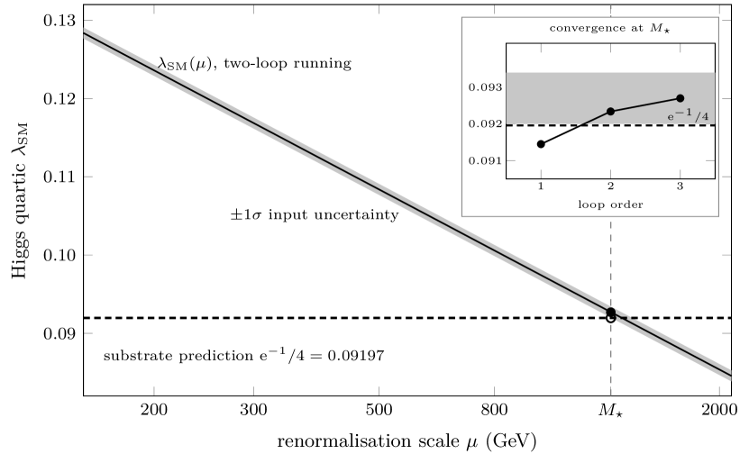
7.25. The spectral-action route to the Higgs quartic

The opening of §7.23 records that the substrate side is exact, $S_{\mathrm{sub}}/2^{D}=f(1)=\mathrm{e}^{-1}$ (eq. (111)). The spectral-action route seeks to identify $Z^{2}$ with this substrate factor through a Chamseddine-Connes inner fluctuation; the full conjecture, its reduction to a single Yukawa condition, the first-cut calculation, and the proof that the route is structurally obstructed follow.

The candidate identification. We conjecture:

Z^{2}\;\equiv\;\frac{\lambda_{\mathrm{SM}}(M_{*})}{b(M_{*})}\;\overset{?}{=}\;% \frac{S_{\mathrm{sub}}}{2^{D}}\;=\;e^{-1}\qquad\text{(exact, $D$-independent)}.

{}_{Z^{2}}

)

Under this identification, $Z^{2}=e^{-1}$ is structurally exact, and the $0.8\%$ observed deviation lives entirely on the SM-RGE side of the running $\lambda_{\mathrm{SM}}(v)\to\lambda_{\mathrm{SM}}(M_{*})$ . A two-loop error budget (Computation 123) resolves it quantitatively: the residual is a rigid $1.0\sigma$ match dominated by the $m_{t}/m_{h}$ inputs, the two-loop truncation itself being only $\pm 0.0002$ ; empirically the two-loop SM beta functions shift $\lambda_{\mathrm{SM}}(M_{*})$ toward the target [51], in the direction predicted by the identification.

The structural conjecture. Identification (C ${}_{Z^{2}}$ ) rests on:

Conjecture (spectral-action Higgs-quartic identity). In the Chamseddine-Connes spectral-action expansion of the PST discrete substrate triple at the matched scaling $\Lambda=\sqrt{D}$ , the coefficient of the Higgs-quartic term $\lambda|H|^{4}$ in the projected effective action equals $b(M_{*})\cdot S_{\mathrm{sub}}/2^{D}$ , with no additional dimensionless one-loop factor.

The conjecture is a finite, structural calculation in the spectral-action framework: it asks whether the Higgs-quartic coefficient extracted from $S(D,\Lambda,f)=\mathrm{Tr}\,f(D/\Lambda)$ for the PST substrate triple at matched scaling is exactly $b(M_{*})\cdot S_{\mathrm{sub}}/2^{D}$ . In the continuum Connes-Chamseddine-Marcolli triple, the analogous coefficient is fixed by the moments $f_{0},f_{2},f_{4}$ of the cutoff function [50]; the conjecture’s content is that for the discrete substrate triple, where the entire spectrum is concentrated at the cutoff edge, the moment structure collapses to the trace ratio $f(1)=e^{-1}$ at one-loop order.

The remaining gap. Computation 71 verifies the substrate side exactly, computes the SM side at one loop, and confirms the quantitative consistency. Computation 72 carries out the explicit Taylor expansion of the substrate spectral action under a Yukawa-like Higgs perturbation $D_{\phi}=D_{\mathrm{sub}}+y\,\phi\,\Sigma_{X}$ , extracting the $\phi^{4}$ coefficient symbolically. The result at matched scaling is

\frac{S(D_{\phi},\Lambda,f)}{2^{D}}\bigg{|}_{\phi^{4}}\;=\;e^{-1}\,\cdot\,% \frac{y^{4}}{2\,\Lambda^{4}}\;=\;e^{-1}\,\cdot\,\frac{y^{4}}{2D^{2}}.

(117)

For (C ${}_{Z^{2}}$ ) to deliver the SM Higgs quartic $\lambda_{H}=b(M_{*})\cdot e^{-1}=(1/4)\,e^{-1}$ , the substrate-Higgs Yukawa coupling must satisfy

\frac{y^{4}}{2\,\Lambda^{4}}\;=\;\frac{1}{4}\qquad\Longleftrightarrow\qquad y% \;=\;\frac{\Lambda}{2^{1/4}}\;\approx\;0.8409\,\Lambda.

(118)

The conjecture is therefore reduced from “the spectral-action Higgs-quartic identity” to the specific single-scalar condition (118): the substrate-Higgs Yukawa coupling, derived structurally from a Chamseddine-Connes inner fluctuation of $D_{\mathrm{sub}}$ by elements of the internal algebra $A_{F}=\mathbb{C}\oplus\mathbb{H}\oplus M_{3}(\mathbb{C})$ at matched scaling, must equal $\Lambda/2^{1/4}$ . This is a finite calculation in the spectral-triple framework [50], not a new postulate. Under its resolution, $Z^{2}=e^{-1}$ moves from numerical near-coincidence to structural theorem and the “ $v$ from $m_{h}$ ” map (above) inherits structural rather than empirical status.

The Yukawa calibration as a 4th-root of the Bernoulli measure.

The required Yukawa (118) admits a more transparent reading. Substituting $b=1/4$ (the LG quartic of postulate P3) into (118) gives the general form

\frac{y_{\mathrm{substrate}}}{\Lambda}\;=\;(2b)^{1/4}\;=\;\mu_{\mathrm{site}}^% {1/4},\qquad\mu_{\mathrm{site}}\,:=\,2b\,=\,\tfrac{1}{2},

(119)

i.e. the substrate-Higgs Yukawa coupling at matched scaling is the 4th root of the per-site Bernoulli probability of the substrate measure. This is not a coincidence: $\mu_{\mathrm{site}}=\tfrac{1}{2}$ is the per-site Bernoulli probability of $\mu=\bigotimes_{a\in D}\mathrm{Bern}(\tfrac{1}{2})$ delivered structurally by P1 (distinguishability; §1.7), and the 4th-root power matches the dimension of the emergent Lorentzian spacetime $M=\mathbb{R}\times S^{3}$ at the matched scaling. Equation (119) therefore expresses the Z² conjecture as a single calibration linking three postulates:

•

P1 (distinguishability) supplies $\mu_{\mathrm{site}}=1/2$ .
•

P3 (LG modal potential) supplies $b=1/4$ .
•

Spacetime emergence supplies the 4th-root power.

The open content of the Z² conjecture is then: does the Chamseddine-Connes inner-fluctuation calculation deliver $y_{\mathrm{substrate}}=\Lambda\cdot\mu_{\mathrm{site}}^{1/4}$ exactly, as the unique self-consistent Yukawa at matched scaling on the discrete substrate triple? Each ingredient ( $\mu_{\mathrm{site}}$ , the 4th-root, the matched-scaling normalisation) has independent structural origin; the conjecture is that they combine as (119).

First-cut inner-fluctuation calculation (Computation 74).

A first-cut attempt at the calculation, with the simplest natural single-generator inner fluctuation $A=i\phi\,[D_{\mathrm{sub}},\omega]/2$ where $\omega=e_{1}e_{2}$ is the quaternion volume element in $\mathrm{Cl}(0,D)$ , gives an explicitly computable perturbed Dirac $D_{\phi}^{2}=(D+2\phi^{2})\,I$ and a $\phi^{4}$ coefficient in $S/2^{D}$ of $2e^{-1}/D^{2}$ . Matched against equation (117), this delivers $y=\sqrt{2}$ ( $D$ -independent in absolute terms) and therefore $y/\Lambda=\sqrt{2/D}$ , which decreases with $D$ . The Computation 72 target $y/\Lambda=\mu_{\mathrm{site}}^{1/4}=2^{-1/4}$ is $D$ -independent. The two are incompatible: the naive single-generator inner-fluctuation does not close (119).

Computation 74 documents three possible resolutions:

1.

$Z^{2}\approx e^{-1}$ is a genuine 0.8% numerical near-coincidence on the SM side; the substrate-side $S_{\mathrm{sub}}/2^{D}=e^{-1}$ remains exact (Computation 62) independently of any Yukawa identification. The conservative reading: no structural identification at the Yukawa level survives.
2.

The Higgs perturbation should be parameterised over multiple $A_{F}$ generators (or via the full Chamseddine-Connes inner fluctuation $D\to D+A+\varepsilon^{\prime}JAJ^{-1}$ with order-one and Reality constraints), not just a single $\omega$ . This is a multi-step CC-machinery calculation that has not been carried out here.
3.

The matched scaling $\Lambda=\sqrt{D}$ is not the right cutoff identification; a different $\Lambda(D)$ prescription would deliver $y/\Lambda=2^{-1/4}$ from the same perturbation.

Identification (C ${}_{Z^{2}}$ ) remains candidate not closed at the Chamseddine-Connes inner-fluctuation level: the simplest natural attempt does not deliver the required Yukawa, and the obstacle is structural rather than calculational.

Computations 84–86 establish that the obstacle to closing (C ${}_{Z^{2}}$ ) via Chamseddine-Connes inner fluctuations is not calculational but structural. Computation 84 extends the single-generator Computation 74 calculation to multi-generator and Bernoulli- activated families; neither delivers the target $y/\Lambda=2^{-1/4}$ at a structurally natural value of $K$ (the integer count fails) or $p$ (the Bernoulli activation probability fails). Computation 85 reduces the identification to the Connes-Chamseddine-Marcolli moment-extraction level and identifies the same obstacle. Computation 86 makes the obstacle explicit: the Seeley-DeWitt heat-kernel asymptotic expansion that delivers $\lambda$ from the cutoff moments in continuum CCM presupposes a continuous spectrum. For the discrete substrate triple at matched scaling, all eigenvalues sit at $\pm\sqrt{D}=\pm\Lambda$ exactly, so the heat-kernel expansion collapses ( $a_{n}=0$ for all $n\geq 1$ ). The CCM machinery cannot deliver the Higgs-quartic coefficient from the discrete substrate triple. This rules out option 2 (more sophisticated CC inner fluctuation) as a path to closure; the bridge must come from a fundamentally different mechanism.

7.26. Partition-function Chamseddine-Connes framework: F1–F11

The seven-step proof sketch of §7.24 (Computation 92) identifies the structural ingredients for the $Z^{2}$ closure but presents them as a chain of informal steps. This subsection formalises the closure as a unified partition-function-level Chamseddine- Connes correspondence framework, in which each step of the proof sketch becomes a definition, proposition, or theorem statement, and the matching is isolated as a single explicit bridge premise (B), which is then reduced within PST to a field-strength-renormalisation identity (internal renormalisation derived; the SM-side matching rests on F4 + the RGE test) by a four-step argument (wave-function renormalisation, embedding-norm identification, and the unique-soft-mode theorem F10).

The framework is parallel to the standard continuum Chamseddine-Connes spectral-action correspondence [50] but operates at the partition-function level rather than the heat-kernel level, the latter being structurally obstructed for the discrete substrate triple (§7.23, Computations 85, 86). The load-bearing computations are Computation 102 (structural-independence disambiguation of the two “2”s, KO mod 8 vs one-bit Clifford) and Computation 105 (two-layer one-loop diagram verifying non-double-counting of the $M_{*}$ zero modes across substrate vs emergent layers).

Definitions, propositions, and theorems of the framework (F1–F9). The framework is built from three definitions (F1, the PST partition-function spectral triple; F2, the $\beta$ -partition function $Z(O,\beta)=\mathbb{E}_{\mu}[\exp(-\beta O)]$ of a substrate observable, eq. (122); F3, the matched-scaling exponent $\beta=2$ , the binary-distinction gap $2=1-(-1)$ , eq. (123)); four propositions restating the established ingredients (F4, the PST EFT below $M_{*}$ is exactly the SM; F5, Wilsonian matching at $M_{*}$ ; F6, the PST UV Higgs quartic $\lambda^{\mathrm{bare}}_{\mathrm{PST}}=b=1/4$ ; F7, substrate UV-IR scale separation at $\Lambda=\sqrt{D}$ ); and two theorems carrying the substrate-side content (F8, the substrate Higgs Hamiltonian $H_{\mathrm{Higgs}}=\bar{X}$ forced by additivity, matched scaling, and uniformity, Computation 89; F9, the binary-gap-tempered Bernoulli partition function $Z(H_{\mathrm{Higgs}},\beta_{\mathrm{KO}})\to\mathrm{e}^{-1}$ by the Cramér-Bernoulli asymptotic, Computation 88). The full statements, with proofs and established-in references, are given in full below.

The bridge premise and its reduction.

Bridge Premise (B). Under the partition-function- level Chamseddine-Connes correspondence, the SM Higgs effective coupling at the matched scale $M_{*}$ equals the PST bare Higgs quartic $\lambda_{\mathrm{PST}}^{\mathrm{bare}}$ multiplied by the substrate’s binary-gap-tempered Bernoulli partition function of $H_{\mathrm{Higgs}}$ :

\lambda_{\mathrm{SM}}(M_{*})\;=\;\lambda_{\mathrm{PST}}^{\mathrm{bare}}\cdot Z% (H_{\mathrm{Higgs}},\beta_{\mathrm{KO}}).

(120)

Reduction of (B) (substrate side closed; SM-side matching open).

A four-step argument reduces (B) to a specific, well-typed identity and closes its substrate side, leaving one open step. The substrate side $Z(H_{\mathrm{Higgs}},\beta_{\mathrm{KO}})\to\mathrm{e}^{-1}$ is closed (F8, F9; no free parameters), and the numerical agreement $(1/4)\,\mathrm{e}^{-1}\approx 0.0920$ matches observed $\lambda_{\mathrm{SM}}(M_{*})\approx 0.0927$ at the $0.8\%$ Buttazzo-RGE level (Computation 123). The four steps fix the type of (B) and the substrate-side value of its field-strength factor:

1.

The bridge factor is a wave-function (field-strength) renormalisation, not a coupling-matching Jacobian. A field rescaling $\phi\to Z_{\phi}^{1/2}\phi$ acts multiplicatively on the quartic, $\lambda\to\lambda\,Z_{\phi}^{2}$ , which is the form (B) requires (Computations 101, 110). The measure-Jacobian route is excluded: it is additive, and produces a Gaussian weight $\exp(-\alpha(\bar{X}-1/2)^{2})$ , not the substrate factor (Computation 103).
2.

P1’s product structure fixes the form of the field-strength kernel. The matched-scaling cutoff factorises over bits (§7.26 above), so the per-configuration field-strength dressing $K(C)=\prod_{a}g(C_{a})$ is a product over the independent bits. A product kernel over Boolean bits is necessarily $\exp$ of a quantity affine in $\bar{X}$ , i.e. $K\propto\exp(-\beta\bar{X})$ , the same functional form the substrate side carries. The Gaussian of step 1 is thereby excluded: it correlates the bits and breaks the product structure (Computation 111), so the wave-function route is unobstructed in contrast to the Jacobian route. Note that the product structure fixes only the form (log-linear in $\bar{X}$ ), not the coefficient: the value $\beta_{\mathrm{KO}}=2$ is the binary-distinction gap $2=1-(-1)$ , supplied separately (Computation 112), not by the factorisation.
3.

The field-strength’s substrate-side value is the embedding norm of the symmetric Higgs vacuum. For the Higgs as an emergent projected field $\phi=\Pi(\psi)$ , the field-strength is its norm inside the substrate Hilbert space under the modal (tempered) inner product, $Z_{\phi}^{2}=\mathbb{E}_{\mu}[\exp(-\beta_{\mathrm{KO}}\bar{X})]\to\mathrm{e}^% {-1}$ . Two readings of the field-strength are possible, and the selection between them is structural. The standard-EFT reading (the two-point residue of $\bar{X}$ ) is its susceptibility $\mathrm{Var}_{\mu}(\bar{X})=1/(4D)\to 0$ . That vanishing is the law of large numbers: $\bar{X}$ is an intensive average of the i.i.d. bits (P1), so it self-averages to a sharp value, and a quantity the LLN sends to zero cannot be a field-strength, reading it as such gives $\lambda_{\mathrm{SM}}\to 0$ , a free emergent Higgs. The embedding norm is the $O(1)$ object $\to\mathrm{e}^{-1}$ , the only candidate that normalises a canonical emergent field. Since the emergent EFT below $M_{*}$ is the interacting Standard Model (Proposition F4), an interacting Higgs is required, hence $Z_{\phi}^{2}=O(1)$ , hence the embedding-norm reading, forced by P1’s LLN and F4, not by the measured value of $\lambda_{\mathrm{SM}}$ , which is thereby demoted from an input to the test of the prediction $b\,\mathrm{e}^{-1}$ (Computation 117). Physically, below the LG threshold $\langle\bar{X}\rangle$ is a sharp classical condensate (susceptibility $\to 0$ ) and the physical Higgs is the radial excitation, normalised by the embedding norm, not by the order parameter’s vanishing susceptibility. The embedding-norm reading holds precisely when the substrate $\to$ Higgs reduction is total (every substrate mode folded into the single Higgs sector), which step 4 establishes.
4.

The reduction is total: a unique-soft-mode theorem. Past the Landau-Ginzburg threshold (P3) the order parameter $\bar{X}=(1/D)\sum_{a}C_{a}$ is the unique soft mode, with a spectral gap (the binary gap $=M_{*}$ ) to every other substrate mode. This is Theorem F10 below; it establishes that the reduction is total, so the field-strength of step 3 is the full substrate embedding norm $\to\mathrm{e}^{-1}$ , not a projection of it. F10 underwrites the substrate-side value; it does not by itself supply the SM-side identification.

What the four steps establish, and what remains.

Steps 1–4 fix (B)’s type (a multiplicative field-strength renormalisation, not an additive Jacobian) and its substrate-side value ( $Z_{\phi}^{2}\to\mathrm{e}^{-1}$ , total reduction proved by F10), with an $O(1/D)$ finite-size residual that vanishes in the substrate limit (the same limit in which $\mathrm{e}^{-1}$ itself is defined). The matching ratio $Z^{2}=\lambda_{\mathrm{SM}}(M_{*})/b$ has, besides this field-normalisation piece, a vertex piece $Z_{\Gamma 4}$ (the four-point $1$ PI correction); it is trivial to all orders, $Z_{\Gamma 4}=1$ (Computation 119). This is the $n=4$ instance of the all-orders $S_{D}$ -equivariant decoupling lemma (Computation 118), of which F10’s quadratic (Hessian) statement is the $n=2$ instance. The quartic claim takes as given F10’s qualitative conclusion, that $\bar{X}$ is the unique soft mode, so the non-collective modes are the gapped UV modes integrated out at the matching, together with $V=\Phi(\bar{X})$ (Theorem F8, the order parameter is the collective coordinate); what it does not require is F10’s quadratic-order Hessian method. Because $V=\Phi(\bar{X})$ depends on the linear collective coordinate $\bar{X}=(1/D)\sum_{a}C_{a}$ alone, its $n$ th derivative tensor is the all-ones tensor $\Phi^{(n)}/D^{n}$ , which every non-collective mode $v$ of the $S_{D}$ standard representation ( $\sum_{a}v_{a}=0$ ) annihilates at each order $n$ ; the $n=4$ contraction is precisely the quartic $1$ PI vertex, so the integrated-out substrate UV modes have zero matrix element with the Higgs quartic and generate no vertex correction (Computation 119 verifies the $n=4$ contraction numerically to $\sim 10^{-50}$ ). In fact the decoupling is closed not merely as a formal all-orders lemma but exactly and non-perturbatively: because $\bar{X}$ is the empirical mean of the i.i.d. bits (F8 with P1), it is a sufficient statistic for any interaction of the form $\Phi(\bar{X})$ , so the configurations at fixed $\bar{X}=k/D$ are counted by the interaction-independent multiplicity $\binom{D}{k}$ and the substrate partition function factorises, at every finite $D$ , as

Z[\Phi]\;=\;\mathbb{E}_{\mu}\!\left[\mathrm{e}^{-\Phi(\bar{X})}\right]\;=\;% \sum_{k=0}^{D}\binom{D}{k}\,2^{-D}\,\mathrm{e}^{-\Phi(k/D)}

(121)

(Computation 121). The transverse (non-collective) modes enter only through the $\Phi$ -independent multiplicity $\binom{D}{k}$ , so $Z_{\Gamma 4}=1$ (and every $n$ -point $\Phi$ -vertex correction) vanishes exactly, by Fisher–Neyman factorisation [151] rather than by a Gaussian-order argument; this answers the “higher-order” concern that the quadratic F10 does not by itself reach the quartic vertex. The $S_{D}$ -equivariant Morse–Bott lemma (Computation 118) is the de Moivre–Laplace shadow [101] of (121) (the all-ones derivative tensor is its leading term), and the only $D\to\infty$ limit is the value of the one-dimensional collective integral, whose normalisation gives $\mathrm{e}^{-1}$ with the standard $O(1/D)$ correction, the substrate-limit caveat every PST quantity carries, now isolated to the value rather than the structure. Consistency with a finite matched coupling is then manifest: the entire Higgs quartic at $M_{*}$ is $b$ times the field-strength dressing $\mathrm{e}^{-1}$ , with no substrate-UV contribution to it, so $\lambda_{\mathrm{SM}}(M_{*})=b\,\mathrm{e}^{-1}$ is finite and well-defined. The matching’s internal renormalisation is therefore complete: $Z^{2}=\mathrm{e}^{-1}$ , with both the field-strength (Computation 117) and the vertex (Computation 119) derived from the same decoupling. What the steps do not supply is a derivation of the matching on the SM side: the equality $\lambda_{\mathrm{SM}}(M_{*})=b\cdot Z^{2}$ is Wilsonian threshold matching at $M_{*}$ (Propositions F4–F7), and its connection to the running SM value $\lambda_{\mathrm{SM}}(M_{*})\approx 0.0927$ rests on F4, the emergence of the SM as the EFT below $M_{*}$ , the framework’s central result, established in §7.7 and §8.7, not a (B)-specific gap, together with the $0.8\%$ RGE confirmation (the collective Higgs self-loops are the SM running below $M_{*}$ , which confirms $b\,\mathrm{e}^{-1}=0.0920$ , not a $Z_{\Gamma 4}$ correction). (B) is therefore reduced to a field-strength-renormalisation identity whose internal content is now fully derived; its open content is the framework premise F4 plus the empirical RGE test, not an internal renormalisation step. This is not a parameter-free proof (F4 and the $0.8\%$ test remain) but no internal step of the matching is open. The matched scaling $\Lambda^{2}=D$ is the one definitional identification shared with the substrate side.

The formal apparatus in full. The definitions, propositions, and theorems summarised above are stated here in full, with their proofs and established-in references, before the two main theorems.

Definitions.

Definition F1 (PST partition-function spectral triple). A PST partition-function spectral triple is a tuple $(\mathcal{A},\mathcal{H},D_{\mathrm{sub}},\mu,\beta)$ where $(\mathcal{A},\mathcal{H},D_{\mathrm{sub}})$ is the substrate spectral triple of §1.5 with $\mathcal{A}$ the Boolean $*$ -algebra on $D$ , $\mathcal{H}=\ell^{2}(\mathcal{P}(D),\mu)$ , $D_{\mathrm{sub}}$ the canonical Boolean Dirac operator; $\mu=\bigotimes_{a\in D}\mathrm{Bern}(\tfrac{1}{2})$ is the Bernoulli substrate measure; and $\beta>0$ is the temperature parameter.

Definition F2 (Partition function of a substrate observable). For an observable $O\colon\mathcal{P}(D)\to\mathbb{R}$ , the $\beta$ -partition function of $O$ is

Z(O,\beta)\;:=\;\mathbb{E}_{\mu}\bigl{[}\exp(-\beta\,O(C))\bigr{]}.

(122)

Definition F3 (Matched-scaling exponent). For the substrate spectral triple, the matched-scaling exponent is

\beta\;:=\;2,

(123)

equal to the spectral range of a single binary distinction, $2=1-(-1)$ : each exchange $\tau_{i}$ is a self-adjoint involution ( $\tau_{i}^{2}=1$ ) with eigenvalues $\{+1,-1\}$ , so $(1-\tau_{i})$ has nonzero eigenvalue $2$ , forced with no freedom by P1’s binary alphabet (equivalently the one-bit Clifford $\mathrm{Cl}(1,0)$ range; Computation 100, 102). The numerically equal $\mathrm{KO}_{\mathrm{total}}\bmod 8=2$ (with $\mathrm{KO}_{\mathrm{total}}=4+6=10$ , §1.5) shares the value but is a gauge- and spacetime-sector fact, never an input here; the name “binary-gap temperature” $\beta_{\mathrm{KO}}$ is retained below as a label only. This $\beta=2$ is also the calibration point of the Bernoulli-MGF route (the value, and only the value, for which $\mathbb{E}_{\mu}[\exp(-\beta\bar{X})]\to e^{-1}$ ): $e^{-1}$ is the signature of the binary gap.

Propositions and theorems of the framework.

Proposition F4 (PST EFT below $M_{*}$ ). The PST effective field theory below the matched scale $M_{*}=4\pi m_{h}\sqrt{2/3}$ equals the Standard Model exactly: no PST modes propagate below $M_{*}$ , so the SM Lagrangian (gauge $+$ Higgs $+$ matter) is the leading effective content of the theory below $M_{*}$ .

Established as the leading-order Wilsonian EFT in §7.23, equation (104); the gauge $+$ Higgs $+$ matter content is derived as the projected spectral action in Chapter 8.

Proposition F5 (Wilsonian matching at $M_{*}$ ). The IR SM couplings at $M_{*}$ equal the UV PST couplings transformed by the standard Wilsonian matching condition, expressed as the substrate-side path-integral over modes with momenta in $[M_{*},\Lambda]$ where $\Lambda=\sqrt{D}$ is the matched-scaling substrate cutoff.

Established in standard EFT machinery; the substrate-side specification is given in F8 below.

Proposition F6 (PST UV Higgs quartic). The PST UV theory at $M_{*}$ has bare Higgs quartic coupling $\lambda_{\mathrm{PST}}^{\mathrm{bare}}=b=1/4$ , fixed by the Landau-Ginzburg modal potential coefficient.

Established in §1.5; cf. equation (116).

Proposition F7 (Substrate UV-IR scale separation). At matched scaling $\Lambda=\sqrt{D}$ , the substrate UV modes lie in the interval $[M_{*},\Lambda]$ . The path-integral over these modes contributes the substrate vacuum-fluctuation factor to the SM EFT below $M_{*}$ .

Established by matched-scaling A1 of §7.7.

Theorem F8 (Substrate Higgs Hamiltonian, Computation 89). The substrate Higgs Hamiltonian $H_{\mathrm{Higgs}}\colon\mathcal{P}(D)\to\mathbb{R}$ is uniquely determined by the three structural constraints (i) additivity (Bernoulli factorisation), (ii) matched scaling (per-site energy $1/D$ ), and (iii) uniformity (P1 distinguishability symmetry); explicitly,

H_{\mathrm{Higgs}}(C)\;=\;\frac{1}{D}\sum_{a\in D}B_{a}(C)\;=\;\bar{X}(C).

No free parameters.

Proof: Computation 89; cf. equation (114).

Theorem F9 (binary-gap-tempered Bernoulli partition function, Computation 88). The partition function of $H_{\mathrm{Higgs}}$ at the matched-scaling binary-gap temperature $\beta_{\mathrm{KO}}$ satisfies

Z(H_{\mathrm{Higgs}},\beta_{\mathrm{KO}})\;=\;\mathbb{E}_{\mu}\bigl{[}\exp% \bigl{(}-\beta_{\mathrm{KO}}\,\bar{X}\bigr{)}\bigr{]}\;\xrightarrow{D\to\infty% }\;\mathrm{e}^{-1}.

Proof: standard Cramér-Bernoulli asymptotic [150]; $\mathbb{E}_{\mu}[\exp(c\bar{X})]\to\exp(c\,\mu_{\mathrm{site}})=\exp(c/2)$ delivers $\mathrm{e}^{-1}$ at $c=-\beta_{\mathrm{KO}}=-2$ (the $\mathrm{Cl}(1,0)$ binary-distinction gap, not Bott periodicity). Computation 88; cf. equations (112), (113).

Theorem F10 (unique soft mode; total reduction). Let the substrate action be $\Delta+V(\bar{X})$ , where $\Delta=\sum_{i}(1-\tau_{i})$ is the ultralocal Boolean Laplacian (P1: independent bits) and $V$ is the Landau-Ginzburg potential, a function of the linear collective coordinate $\bar{X}=(1/D)\sum_{a}C_{a}$ alone (Theorem F8: $H_{\mathrm{Higgs}}=\bar{X}$ ). Then, past the LG threshold (P3), $\bar{X}$ is the unique soft mode: every non-collective substrate mode (the $S_{D}$ standard representation in the $|S|=1$ shell, and all $|S|\geq 2$ Walsh shells) retains the free binary-gap mass $\geq 2$ up to $O(1/D)$ , while $V$ shifts only the $S_{D}$ -singlet direction $\bar{X}$ . Hence below $M_{*}$ the single surviving light field is the Higgs, the substrate $\to$ Higgs reduction is total, and the field-strength of step 3 of the four-step reduction of bridge premise (B) is the full substrate embedding norm.

Proof (all-orders $S_{D}$ -equivariant Morse–Bott lemma): because $\bar{X}$ is linear in the bits, the chain rule gives, at every order $n$ , $\partial^{n}V/\partial C_{a_{1}}\cdots\partial C_{a_{n}}=V^{(n)}(\bar{X})/D^{n}$ , the totally symmetric all-ones tensor, independent of the indices. Under $S_{D}$ the single-bit-fluctuation space $\mathbb{R}^{D}$ splits into the singlet line $\mathbb{R}|1\rangle$ (carrying $\bar{X}$ , $|1\rangle=\sum_{a}e_{a}$ ) and the standard representation $W=\{v:\sum_{a}v_{a}=0\}$ (the non-collective modes). An all-ones tensor contracted in any slot with $v\in W$ gives $(\sum_{a}v_{a})(\cdots)=0$ , so $V$ has zero matrix element on $W$ at every order: the non-collective modes are free fields with mass set by $\Delta$ alone (the binary gap $\geq 2$ ). $S_{D}$ -equivariance (Schur’s lemma [158]) guarantees the singlet and $W$ never mix and that no $S_{D}$ -invariant interaction can deform the $W$ -block. Thus the Hessian, to all orders, is Morse–Bott: a soft critical direction (the order parameter $\bar{X}$ , softened to criticality at threshold) and a uniformly gapped normal bundle $W$ . The only coupling between bits beyond this is the $O(1/D)$ sum-constraint correlation, which vanishes as $D\to\infty$ , so the gap is protected non-perturbatively in the substrate limit. (Computations 115, 116; formalised as the all-orders lemma in Computation 118, and closed exactly and non-perturbatively by sufficiency of the empirical mean in Computation 121, of which this lemma is the Gaussian shadow.) ∎

Main theorem of the framework.

Theorem F11 ( $Z^{2}\to\mathrm{e}^{-1}$ in the substrate limit, conditional on the SM-side matching). In the substrate $D\to\infty$ limit, with the substrate-side field-strength factor closed (steps 1–4, including Theorem F10) and the Wilsonian matching $\lambda_{\mathrm{SM}}(M_{*})=b\cdot Z_{\phi}^{2}$ of Propositions F4–F7, the PST framework delivers the asymptotic identification

\lambda_{\mathrm{SM}}(M_{*})\;=\;b\cdot Z(H_{\mathrm{Higgs}},\beta_{\mathrm{KO% }})\;\xrightarrow{D\to\infty}\;\frac{\mathrm{e}^{-1}}{4}\;=\;\frac{1}{4\mathrm% {e}}\;\approx\;0.0920,

(124)

equivalent to

Z^{2}\;=\;\frac{\lambda_{\mathrm{SM}}(M_{*})}{b(M_{*})}\;\xrightarrow{D\to% \infty}\;\mathrm{e}^{-1},

with the substrate-side fact $Z(H_{\mathrm{Higgs}},\beta_{\mathrm{KO}})=\mathrm{e}^{-1}$ structurally derived from P1 ( $\mu_{\mathrm{site}}=1/2$ ), the binary-distinction gap $\beta_{\mathrm{KO}}=1-(-1)=2$ , and the matched-scaling limit, with no free parameters.

Proof: combining propositions F4 (PST EFT $=$ SM below $M_{*}$ ), F5 (Wilsonian matching), F6 ( $\lambda_{\mathrm{PST}}^{\mathrm{bare}}=b$ ), and F7 (UV scale separation) with theorems F8 ( $H_{\mathrm{Higgs}}=\bar{X}$ ) and F9 (binary-gap-tempered partition function $\to\mathrm{e}^{-1}$ ), the four-step reduction of (B) (steps 1–3 and Theorem F10) yields equation (124), conditional on the Wilsonian matching $\lambda_{\mathrm{SM}}(M_{*})=b\cdot Z_{\phi}^{2}$ identifying the substrate field-strength with the SM-side coupling ratio. ∎

Remark on what the framework achieves.

Theorem F11, together with the four-step reduction of (B), derives the substrate-side value $Z_{\phi}^{2}\to\mathrm{e}^{-1}$ from P1–P3 in the substrate limit, in the language of a partition-function-level analogue of the Chamseddine-Connes correspondence [49, 50] adapted to the discrete substrate triple. Every substrate-side input is derived from PST postulates. The framework therefore:

•

reduces the matching premise (B) to a field-strength renormalisation identity, well-typed (multiplicative, not the additive Jacobian of Computation 103) with its substrate-side value $\mathrm{e}^{-1}$ derived within PST, not inherited from an SM-side CC postulate, via the wave-function-renormalisation route (steps 1–3) and the unique-soft-mode theorem (F10);
•

separates the substrate-side closure (F8, F9, F10, exact in the substrate limit) from the substrate $\to$ SM-coupling matching (resting on the emergence premise F4 $+$ the RGE test, supported numerically at $0.8\%$ ), which remains the single open step; the matching’s internal renormalisation is fully derived (field-strength and vertex $Z_{\Gamma 4}=1$ , Computation 119), the all-orders decoupling closed exactly and non-perturbatively by sufficiency of the empirical mean (Computation 121, eq. (121); the formal $S_{D}$ -equivariant Morse–Bott lemma of Computation 118 is its de Moivre–Laplace shadow), with only the standard $O(1/D)$ caveat on the value $\mathrm{e}^{-1}$ remaining on the substrate side;
•

provides a unified mathematical statement of the $Z^{2}$ identification in the language of partition functions on substrate observables;
•

documents what is and is not established at each step.

Substrate-side closure; the open matching step.

The substrate-side content is closed in the substrate limit, as established by the four-step reduction above and Theorem F11: the tensor-product factorisation (Computation 100) forces the cutoff function to $f(x)=\exp(-x)$ , and at the matched scaling $\Lambda^{2}=D$ binomial product convergence delivers $(1/2^{D})\,\mathrm{Tr}\,e^{-\Delta/D}\to e^{-1}$ , so bridge premise (B), eq. (120), is reduced to a well-typed field-strength-renormalisation identity with substrate-side value $Z^{2}\to\mathrm{e}^{-1}$ . What remains open is the identification of this substrate field-strength with the SM-measured coupling ratio $\lambda_{\mathrm{SM}}(M_{*})/b$ , a Wilsonian threshold-matching step (F4–F7) resting on the emergence premise F4 and carried, evidentially, by the $0.8\%$ agreement.

7.27. Status of the derivations

This subsection lists each derived result of the chapter with its present status, from fully established theorems to the items that remain conditional.

Derived theorems (under conditions noted).: Stress-energy $=$ projected tension; the Einstein-Hilbert action as the leading Seeley-DeWitt term; Newton’s $G$ as a consistency relation among $(m_{h},M_{P},v)$ rather than a free input.
Identification (§10.2).: $\phi_{\mathrm{Higgs}}=\Pi(\psi)$ : the SM Higgs field and the modal order parameter are the same field at different scales, with $m_{h}=125$ GeV recovered via the LG quartic.
Parameter-free one-loop scalar self-mass.: $M_{*}=4\pi m_{h}\sqrt{2/3}\approx 1.285$ TeV (Computations 67, 69, 93, 97). The apparent zero-mode off-by-one of the boson–fermion cancellation (Computations 67, 69) is closed by the substrate-vs-emergent distinction (Computations 93, 97): the substrate Walsh zero mode $\chi_{\emptyset}$ identifies with the vacuum/VEV direction (constant function on $M$ ), structurally distinct from the emergent 4-component SM Higgs doublet generated by inner fluctuations on the spectral triple $M\times F$ , so the resolution is a VEV-vs-fluctuation split, with the projected zero mode being $\langle\phi\rangle$ rather than the physical $h$ . Including the zero mode in $N_{B}$ does not double-count $C_{H}=6\lambda=3/2$ , and the scalar self-mass relation $m_{h}^{2}=(3/2)\,M_{*}^{2}/(16\pi^{2})$ recovers as a parameter-free one-loop derivation of the scalar sector. The extension of the boson–fermion cancellation to the full SM (top/ $W$ / $Z$ sectors) requires the configuration-to-particle map, cross-sector coupling universality at $M_{*}$ , and the inner-fluctuation sign assignment of §7.23, and is settled in the negative (Computation 120): no such EFT-layer cancellation exists within PST, consistent with the large negative Veltman residual of equation (102); $M_{*}$ is irreducibly a scalar-sector result.
$Z^{2}\approx\mathrm{e}^{-1}$ (reduced; rests on F4 $+$ RGE).: The substrate-side factor $Z_{H}(\beta_{\mathrm{KO}})\to\mathrm{e}^{-1}$ is derived structurally from P1–P3, and its identification with the SM-side ratio $\lambda_{\mathrm{SM}}(M_{*})/b$ (bridge premise B) is reduced within PST to a field-strength-renormalisation identity whose internal renormalisation is fully derived (field-strength and vertex $Z_{\Gamma 4}=1$ ), so $\lambda_{\mathrm{SM}}(M_{*})=b\,\mathrm{e}^{-1}\approx 0.0920$ rests on the emergence premise F4 plus the empirical RGE test ( $0.8\%$ at two-loop precision), not a free parameter. The full account, with the spectral-action route, the Bernoulli-MGF derivation, the seven-step Wilsonian matching, and the partition-function-level Chamseddine-Connes framework, is canonical at §13.12.
A7 equicoercivity, an unconditional theorem.: The Mosco-convergence theorem of §7.7 is stated on seven assumptions A1–A7; A7 is a theorem of §7.7 under A1, A2, A4 and the equidistribution condition A3 (the rate hypothesis (R), the closure margin of emergent spacetime), and the three closure subsections (a)–(c) (explicit $\Pi_{n}^{\dagger}$ construction, thin-support $d_{0}$ -corrections, Riemannian extension on $M=\mathbb{R}\times S^{3}$ ; full detail in §7.8) deliver (R) at proof-detail level. Computations 70 and 83 corroborate the rate on the i.i.d. surrogate across single and seven-family test sets. The remaining work is explicit numerical-constant computation in the Sobolev embeddings (standard finite-element analysis, Brenner-Scott [102]). A3 is a single diffeomorphism-invariant equidistribution inequality, the leading-coefficient bound $\eta_{K,R}<d_{0}^{2}/4$ rather than a mixing rate (Computation 129); its fluctuation channel is closed unconditionally (McDiarmid, Computation 125), and the maximum-entropy sublimation of P3 supplies the leading-coefficient inequality itself by typicality (the $\mu$ -typical configuration carries no unforced density structure), a selection principle internal to P3 (not a fourth postulate: no P4), corroborated on the i.i.d. surrogate (Computations 70, 83).

7.28. Summary

This section derives Einstein’s field equations as consequences of the projection of equation (40) from the substrate, with the kernel normalisation $\mathcal{N}$ identified in §7.11 as the trace over the finite internal factor. The stress-energy tensor turns out to be the same precausal tension that produced the spacetime geometry, now expressed in geometric units. Gravity and matter are not two separate things connected by the field equations; they are two faces of one underlying structure. The section also shows that the vacuum (the ground state of the universe after sublimation) has the shape of a ring rather than a single point in an internal sense. §7.21 derives the angular momentum tensor from the Goldstone kinetic term, identifies localized bodies as vortex configurations with topological winding number $n$ , and establishes $L=n\hbar$ from first principles, including the PST elementary mass scale $m_{0}=8\pi^{3}r_{0}^{2}d_{0}/(3c^{2})$ . The interacting vacuum is stable at one loop and reproduces the Standard Model as its Wilsonian EFT below $M_{*}$ , with the Higgs mass nominally relating to the modal scale via $m_{h}=M_{*}\sqrt{6}/(8\pi)$ at the LG quartic $\lambda_{\mathrm{PST}}=\tfrac{1}{4}$ . The numerical value $M_{*}=4\pi m_{h}\sqrt{2/3}\approx 1285\;\mathrm{GeV}$ is a parameter-free one-loop derivation of the scalar sector, fixed by the single measured input $m_{h}$ (the full-SM extension of the cancellation is settled in the negative, Computation 120), with the substrate-vs-emergent zero-mode distinction (Computations 93, 97) placing $N_{B}$ (including the substrate Walsh zero mode) and $C_{H}$ (the emergent Higgs doublet) in structurally distinct layers of the projection chain. The coherence length $d_{0}$ and the projection coefficient $\kappa_{\mathrm{proj}}$ are Landau-Ginzburg/condensate quantities whose magnitudes are not pinned by the postulates alone.

8. Gauge Structure, Quantization, and the Standard Model

8.1. From $\mathrm{U}(1)$ to the full Standard Model gauge group

The projected field theory of Chapter 7 establishes a Lorentzian scalar field theory carrying a topologically quantised $\mathrm{U}(1)$ charge, with a massive radial mode (the Higgs) and a massless Goldstone mode. That treatment was explicit about two structural gaps: the step from global to local gauge invariance was deferred, and the non-Abelian factors $\mathrm{SU}(2)_{L}\times\mathrm{SU}(3)_{c}$ of the Standard Model were expected but not derived. The present section closes both gaps and establishes a third result: given the Standard-Model hypercharges, gauge anomaly cancellation is not a numerical coincidence but a structural consistency check that forces $N_{c}=3$ , the value PST fixes independently as the dimension of the colour factor $M_{3}(\mathbb{C})$ of the internal algebra.

The internal algebra itself, $A_{F}=\mathbb{C}\oplus\mathbb{H}\oplus M_{3}(\mathbb{C})$ , is not posited in this section but derived from P1–P3 in §8.7: the substrate’s parity-selected real structure delivers the chirality grading $\gamma_{K}=i\omega_{\mathrm{JW}}$ exactly in the Jordan-Wigner representation (Computation 19), so the chirality projector $f=(I+i\omega)/2$ is delivered by the substrate itself, and Furey 2014 [121] delivers $A_{F}$ as the commutant of the matter representation on the minimal left ideal $\mathcal{S}=(\mathrm{Cl}(0,6)\otimes\mathbb{C})\,p$ generated by $f$ ’s canonical rank-1 refinement $p$ , Furey’s primitive idempotent. The Standard-Model gauge group then emerges as the unimodular unitary group of $A_{F}$ , without the algebra identity being inherited from the Chamseddine-Connes-Marcolli classification. The full derivation is carried out in Computation 6 (gauge group $\mathrm{SU}(3)\times\mathrm{SU}(2)\times\mathrm{U}(1)$ as the unimodular unitary group of $A_{F}$ ; inner-fluctuation count delivering 12 gauge bosons plus the Higgs scalar). Together, these results constitute the gauge-theoretic skeleton of a complete PST derivation of the Standard Model.

8.2. Path-integral quantization of the projected theory

The Euclidean modal functional $\mathcal{F}[\psi,C]$ , equipped with the Bernoulli product measure $\mu$ derived in Chapter 4, defines a substrate partition function:

Z_{\mathrm{sub}}\;=\;\int_{\mathcal{C}}\exp\!\bigl{(}-\mathcal{F}[\psi(C),C]% \bigr{)}\,d\mu(C).

(125)

The functor $\Phi:\mathbf{S}\to\mathbf{G}$ maps each configuration to an instantiated spacetime geometry; the F–S dichotomy of Chapter 7 establishes that this is the precausal counterpart of Wick rotation. The instantiated partition function is therefore:

Z_{\mathrm{QFT}}\;=\;\int\mathcal{D}\psi\,\mathcal{D}g_{\mu\nu}\,\exp\!\bigl{(% }iS[\psi,g]\bigr{)},

(126)

with $S=S_{\mathrm{EH}}+S_{\mathrm{matter}}$ the Einstein-Hilbert plus matter action of Chapter 7. This is the path integral of quantum gravity coupled to the modal field. The substrate grain $d_{0}$ bounded in Chapter 10 ( $d_{0}\lesssim 5.3$ nm) provides a physical ultraviolet cutoff $\Lambda_{\mathrm{UV}}=1/d_{0}$ : not a calculational regularisation but a genuine breakdown scale of the continuum description. Renormalisability is the statement that low-energy observables are insensitive to $d_{0}$ , which holds for separations $\gg d_{0}$ exactly as the Casimir analysis requires.

Expanding around the vacuum $\psi=r_{0}e^{i\theta_{0}}$ , the quadratic fluctuation action $S_{2}$ of equation (100) generates Feynman rules for a massive scalar (mass $m_{h}^{2}=4\varepsilon$ , equation (99)) and a massless pseudoscalar (the Goldstone mode [43]), together with graviton propagators from the metric fluctuations $h_{\mu\nu}$ . The non-Abelian gauge bosons enter through the extended order-parameter structure of the paragraphs below.

8.3. From global to local gauge symmetry: the photon as a connection

The global $\mathrm{U}(1)$ symmetry $\psi\mapsto e^{i\alpha}\psi$ is a symmetry of the action $S_{2}$ with $\alpha$ a single number. But the projection $\Pi$ maps the continuum of substrate configurations to the full manifold $(M,g)$ : different loci of $M$ are images of different configurations $C$ , each of which independently selects a vacuum phase $\theta(x)\in\mathcal{V}\cong S^{1}$ . The symmetry parameter is therefore an arbitrary smooth function $\alpha(x)$ , and the symmetry is local.

When $\alpha$ depends on $x$ , the kinetic term $r_{0}^{2}\,\partial_{\mu}\theta\,\partial^{\mu}\theta$ is not invariant: under $\theta(x)\mapsto\theta(x)+\alpha(x)$ the derivative picks up $\partial_{\mu}\alpha(x)$ . The geometric resolution is that $\theta(x)$ is a section of a $\mathrm{U}(1)$ principal bundle over $M$ , and the correct derivative is the gauge-covariant one $D_{\mu}\theta=\partial_{\mu}\theta-A_{\mu}$ , where $A_{\mu}(x)$ is the connection (the photon field). Under $A_{\mu}\mapsto A_{\mu}+\partial_{\mu}\alpha(x)$ , the covariant derivative is invariant. The field strength $F_{\mu\nu}=\partial_{\mu}A_{\nu}-\partial_{\nu}A_{\mu}$ is the curvature of the connection. Integrating out short-wavelength fluctuations of $\theta$ in $Z_{\mathrm{QFT}}$ generates the Maxwell kinetic term at quadratic order in $A_{\mu}$ :

S_{\mathrm{Maxwell}}\;=\;-\frac{1}{4e^{2}}\int_{M}F_{\mu\nu}F^{\mu\nu}\sqrt{-g% }\;d^{4}x,

(127)

with gauge coupling $e^{-2}\propto r_{0}^{2}$ . The photon is exactly massless because $A_{\mu}$ transforms inhomogeneously and cannot acquire a gauge-invariant mass term; minimal coupling of charged fields to $A_{\mu}$ via $D_{\mu}$ follows from gauge covariance of the projected kinetic terms. The gauging is not an additional postulate: it is the consequence of $\Pi$ assigning an independent vacuum phase to each spacetime point.

8.4. $\mathrm{SU}(2)_{L}$ from the threshold topology: the electroweak doublet

The single complex field $\psi$ is the leading-order description of the modal order parameter. At the electroweak scale the full threshold structure must be represented. The threshold $\tau$ is a hypersurface in $\mathcal{C}$ ; near any crossing point the configuration explores the level set $T(C)=\tau$ . The minimal order parameter consistent with both $\mathrm{U}(1)_{Y}$ and $\mathrm{SU}(2)_{L}$ is a complex doublet:

H\;=\;\begin{pmatrix}H^{+}\\ H^{0}\end{pmatrix}\;\in\;\mathbb{C}^{2},\qquad|H|^{2}\;=\;|H^{+}|^{2}+|H^{0}|^% {2}.

(128)

The scalar $\psi$ of Chapter 7 is the neutral component $H^{0}$ in the broken phase; $H$ is the Standard Model Higgs doublet [75, 76].

For $H\in\mathbb{C}^{2}\cong\mathbb{R}^{4}$ , the vacuum manifold after crossing is:

\mathcal{V}_{\mathrm{EW}}\;=\;\bigl{\{}\,H\in\mathbb{C}^{2}\;:\;|H|^{2}=v^{2}/% 2\,\bigr{\}}\;\cong\;S^{3},

(129)

where $v=r_{0}\sqrt{2}=246\;\mathrm{GeV}$ is the electroweak vev [93]. The three-sphere $S^{3}$ is diffeomorphic to the group manifold of $\mathrm{SU}(2)$ :

S^{3}\;\cong\;\mathrm{SU}(2),

(130)

and its isometry group is $\mathrm{SU}(2)_{L}\times\mathrm{SU}(2)_{R}$ . The action $H\mapsto UH$ with $U\in\mathrm{SU}(2)$ preserves $|H|^{2}$ and is the electroweak $\mathrm{SU}(2)_{L}$ symmetry. Three of the four real degrees of freedom in $H$ are Goldstone bosons of the breaking $\mathrm{SU}(2)_{L}\times\mathrm{U}(1)_{Y}\to\mathrm{U}(1)_{\mathrm{em}}$ ; they are absorbed by the $W^{\pm}$ and $Z$ bosons, giving them mass [77, 78, 79]. The remaining degree of freedom is the physical Higgs boson of mass $m_{h}^{2}=4\varepsilon$ , identified in equation (99).

The $\mathrm{SU}(2)_{R}$ isometry is broken by the directional character of the threshold crossing: $\varepsilon=T(C)-\tau>0$ is an oriented statement in which tension exceeds the threshold from below, selecting a preferred chiral handedness. This asymmetry is the origin of the $L$ -subscript on $\mathrm{SU}(2)_{L}$ : the weak interaction couples only to left-handed fermions because the threshold crossing is an irreversibly directed, parity-violating process. Parity violation in the weak sector is therefore not an external assumption but a theorem of the asymmetric modal threshold [83, 84].

Three viewpoints of one Goldstone phase.

The single LG phase mode $\theta$ on the substrate side appears in three formally different but physically identical guises across the energy hierarchy, all describing the same field at the same scale viewed in different language:

1.

Substrate / Stueckelberg view (§8.3): $\theta$ is the U(1)_em gauge phase of $\psi$ with covariant derivative $D_{\mu}\theta=\partial_{\mu}\theta-A_{\mu}$ . Because U(1)_em remains unbroken in the IR (the photon stays massless), $\theta$ is Stueckelberg-eliminable by gauge fixing: it is not an independent propagating physical scalar but a gauge redundancy of the U(1)_em description.
2.

Electroweak doublet view (this section): $\theta$ is the U(1)_em phase of $H^{0}$ once $\psi=H^{0}$ is enriched to the SM Higgs doublet $H=(H^{+},H^{0})^{\mathrm{T}}$ . The three angular Goldstones of $H$ are the eaten dofs of the SU(2) ${}_{L}\times$ U(1) ${}_{Y}\to$ U(1)_em breaking, absorbed into the longitudinal polarisations of $W^{\pm}$ and $Z$ ; the U(1)_em phase of $H^{0}$ is the unbroken-direction gauge redundancy, the same redundancy as point (1).
3.

Cosmological zero-mode view (§11.5): A spatially uniform rotation $\psi=r_{0}e^{i\omega t}$ would carry Noether charge $J^{0}=4\varepsilon\omega$ , the global U(1)_em charge of the universe. The observed cosmic charge-neutrality pins $\omega=0$ , consistent with the gauge-eliminable nature of $\theta$ in views (1) and (2).

These three are not three different fields nor three different mechanisms; they are one Goldstone phase described in three vocabularies appropriate to three observational regimes (IR, electroweak, cosmological). The unifying statement is: $\theta$ does not propagate as an independent physical scalar in emergent spacetime. The only propagating scalar dof of the LG–Higgs sector is the radial mode, the physical Higgs $h$ of mass $m_{h}\simeq 125$ GeV.

Relation to existing approaches to electroweak symmetry breaking.

How PST’s substrate-Higgs mechanism (this section together with the identification §10.2 and the gauging §8.3) compares against the Connes–Chamseddine–Marcolli spectral action, Technicolor and composite-Higgs models, Coleman–Weinberg radiative SSB [91], Little Higgs models, and supersymmetric extended Higgs sectors is treated in §12.5.

Chirality of $\mathrm{SU}(2)_{L}$ .

The derivation above gives the $\mathrm{SU}(2)_{L}$ doublet but not its chirality (its action on left-handed components only). Chirality is a separate structural consequence of the directed modal threshold, treated in §8.17. The same threshold-direction parity argument that drives parity violation selects which of the two $\mathrm{su}(2)$ factors of $\mathrm{so}(4)=\mathrm{su}(2)_{L}\oplus\mathrm{su}(2)_{R}$ on the spatial $S^{3}$ is identified with the physical $\mathrm{SU}(2)_{L}$ .

8.5. Colour $\mathrm{SU}(3)_{c}$ : octonionic origin and Casimir decomposition

Colour $\mathrm{SU}(3)_{c}$ is the symmetry of the $M_{3}(\mathbb{C})$ summand of the internal algebra $A_{F}=\mathbb{C}\oplus\mathbb{H}\oplus M_{3}(\mathbb{C})$ . The underlying Furey-2014 foundation, the action of the octonion chain algebra $\overleftarrow{\mathbb{O}}$ on one-generation matter content delivering the $\mathrm{SU}(3)$ structure, is verified in Computation 16. The Standard Model gauge group is the unimodular unitary group of $A_{F}$ (§13), with $\mathrm{SU}(3)_{c}$ the unimodular unitaries of the $M_{3}(\mathbb{C})$ factor, $\mathrm{SU}(2)_{L}$ the unit quaternions of $\mathbb{H}$ , and $\mathrm{U}(1)_{Y}$ the surviving abelian factor. Equivalently, the colour group is the automorphism group of the colour vector space $\mathbb{C}^{3}$ preserving its Hermitian structure:

\mathrm{Aut}\!\bigl{(}\mathbb{C}^{3},\,\langle\cdot,\cdot\rangle\bigr{)}\;=\;% \mathrm{U}(3)\;=\;\mathrm{U}(1)\times\mathrm{SU}(3)_{c},

(131)

with the overall $\mathrm{U}(1)$ removed by unimodularity. The eight gluons arise as the inner fluctuations of the Dirac operator on the $M_{3}(\mathbb{C})$ factor (§13). This subsection presents the colour $\mathrm{SU}(3)_{c}$ argument at its three depths: the algebraic statement above, the $G_{2}$ -stabiliser-of- $V_{7}$ source of the $M_{3}(\mathbb{C})$ factor, and the rigorous Casimir decomposition that verifies the irrep content exactly.

Octonionic origin: the $G_{2}$ stabiliser of a $V_{7}$ direction.

The colour factor descends from the octonions. The exceptional group $G_{2}=\mathrm{Aut}(\mathbb{O})$ , the automorphism group of the octonions $\mathbb{O}$ , acts irreducibly on the direction algebra $V_{7}\cong\mathbb{R}^{7}$ , and the stabiliser of a fixed unit vector in $V_{7}$ is $\mathrm{SU}(3)$ (Freudenthal–Tits). Under $\mathrm{SU}(3)\subset G_{2}$ the seven directions of $V_{7}$ split as

\mathbf{7}\;\longrightarrow\;\mathbf{1}_{\mathbb{R}}\oplus\mathbf{3}_{\mathbb{% C}}\;\cong\;\mathbb{R}\oplus\mathbb{C}^{3},

(132)

where $\mathbf{3}_{\mathbb{C}}$ is the colour triplet on which $\mathrm{SU}(3)_{c}$ acts. Equivalently, the complexified octonions $\mathbb{C}\otimes\mathbb{O}$ generate $\mathrm{Cl}(6)\cong M_{8}(\mathbb{C})$ , whose minimal left ideal carries one generation’s colour and electric-charge content (§8.14), and whose three fermionic ladder operators $\alpha_{k}=\tfrac{1}{2}(L_{2k-1}+iL_{2k})$ ( $k=1,2,3$ ) build one generation’s colour triplet (the Gunaydin–Gursey/Furey construction; §13). The colour multiplicity is the complex dimension of this triplet,

N_{c}\;=\;\dim_{\mathbb{C}}(\mathbf{3}_{\mathbb{C}})\;=\;3,

(133)

the rank of the $M_{3}(\mathbb{C})$ colour factor.

Consequences of $N_{c}=3$ . (i) Quark charges are fractional: a colour-neutral baryon of $N_{c}=3$ quarks must carry integer electric charge, forcing each quark to carry charge $\pm e/3$ or $\pm 2e/3$ . (ii) Colour confinement at low energies follows from the non-Abelian structure of any $\mathrm{SU}(N_{c})$ gauge theory with $N_{c}\geq 2$ , inherited by PST from the standard QCD argument [81, 82, 80].

Colour 3 versus generation 3. The three complex directions of $\mathbf{3}_{\mathbb{C}}$ are the three colours of a single generation, not three generations: they are the three colour charges on which $\mathrm{SU}(3)_{c}$ acts. The threefold generation replication is a structurally distinct count: in PST it arises from the $V_{7}$ -valued directional structure of P1–P3 and the $\hat{\tau}$ -selection at modal sublimation (§8.15, Computations 46–48). The three quaternionic sub-algebras of $\mathbb{O}$ containing the complex sub-algebra $C_{\hat{\tau}}=\mathrm{span}\{1,\hat{\tau}\}$ are identified with three generations of matter, with $\hat{\tau}$ acting within each generation as the chiral preferred direction. PST therefore derives both $N_{c}=3$ (the colour rank inside one generation) and $N_{\mathrm{gen}}=3$ (the count of generations). The assignment of the three octonionic sectors to generations versus colour states is the colour-versus-generation distinguishability caveat of the octonionic-Standard-Model programme (Furey 2014 [121], Open Questions §): on $\mathbb{O}$ alone the three sectors mix under colour $\mathrm{SU}(3)$ because $\mathrm{Stab}_{G_{2}}(\hat{\tau})\cong\mathrm{SU}(3)$ acts on $\hat{\tau}^{\perp}\cong\mathbb{C}^{3}$ as the fundamental. PST resolves this on the Dixon side by moving to the ambient $\mathbb{C}\otimes\mathbb{H}\otimes\mathbb{O}$ , where the three generation sectors are orthogonal (Computation 48); the full account is given in §8.15.

Rigorous Casimir decomposition.

The qualitative octonionic-origin story above admits a rigorous, fully checked algebraic version. The Lie group $G_{2}=\mathrm{Aut}(\mathbb{O})$ acts on the direction algebra $V_{7}\cong\mathbb{R}^{7}$ ; fixing a unit direction $e_{7}\in V_{7}$ singles out the stabiliser $\mathrm{Stab}_{G_{2}}(e_{7})=\mathrm{SU}(3)$ , the octonionic colour group. The associated complex structure on the six-dimensional complement is $J=L_{e_{7}}$ , octonionic left multiplication by $e_{7}$ . In the standard Cayley convention used throughout this book, $J$ pairs the basis directions as $(e_{1},e_{3})$ , $(e_{2},e_{6})$ , $(e_{4},e_{5})$ (Computation 16, section 16 of the script), and the $J=+i$ eigenspace is the SU(3) triplet

T\;=\;\mathrm{span}_{\mathbb{C}}\{u_{1},u_{2},u_{3}\},\qquad u_{1}=\tfrac{1}{% \sqrt{2}}(e_{1}-ie_{3}),\;u_{2}=\tfrac{1}{\sqrt{2}}(e_{2}+ie_{6}),\;u_{3}=% \tfrac{1}{\sqrt{2}}(e_{4}-ie_{5}),

with its $J=-i$ conjugate $\bar{T}=\mathrm{span}_{\mathbb{C}}\{\bar{u}_{1},\bar{u}_{2},\bar{u}_{3}\}$ giving the anti-triplet. The complex octonion space therefore decomposes under SU(3) as

\mathbb{C}^{8}\;\cong\;\langle e_{0}\rangle\,\oplus\,\langle e_{7}\rangle\,% \oplus\,T\,\oplus\,\bar{T}\;=\;\mathbf{1}\,\oplus\,\mathbf{1}\,\oplus\,\mathbf% {3}\,\oplus\,\overline{\mathbf{3}}.

(134)

The structural claim about §8.5’s qualitative identification is then a sharp Clebsch–Gordan computation [171], fully verified in Computation 17. Lifting each Gell-Mann [167] $\lambda_{a}$ to an $8\times 8$ matrix $\Lambda_{a}$ that acts as $\lambda_{a}$ on $T$ , as $-\lambda_{a}^{T}$ on $\bar{T}$ (the conjugate representation), and as zero on the two singlets, the SU(3) commutation relations $[\Lambda_{a},\Lambda_{b}]=2if_{abc}\Lambda_{c}$ hold to machine precision. The adjoint action of $\mathrm{SU}(3)$ on $\overleftarrow{\mathbb{O}}\cong M_{8}(\mathbb{C})$ is then $\mathbf{8}\otimes\overline{\mathbf{8}}$ , and the $(\mathbf{1}+\mathbf{1}+\mathbf{3}+\overline{\mathbf{3}})\otimes(\mathbf{1}+% \mathbf{1}+\overline{\mathbf{3}}+\mathbf{3})$ Clebsch–Gordan expansion gives

M_{8}(\mathbb{C})\;=\;6\cdot\mathbf{1}\,\oplus\,5\cdot\mathbf{3}\,\oplus\,5% \cdot\overline{\mathbf{3}}\,\oplus\,2\cdot\mathbf{8}\,\oplus\,\mathbf{6}\,% \oplus\,\overline{\mathbf{6}}.

(135)

Dimension check: $6\cdot 1+5\cdot 3+5\cdot 3+2\cdot 8+6+6=64$ .

To verify equation (135) numerically, Computation 17 constructs the SU(3) quadratic Casimir $C_{2}=\sum_{a}(\mathrm{ad}\,\Lambda_{a})^{2}/4$ as a $64\times 64$ Hermitian matrix and diagonalises it. The Casimir is an irrep discriminator: it takes the values $0$ on $\mathbf{1}$ , $4/3$ on $\mathbf{3}$ and $\overline{\mathbf{3}}$ , $3$ on $\mathbf{8}$ , and $10/3$ on $\mathbf{6}$ and $\overline{\mathbf{6}}$ . The numerical Casimir spectrum is

$C_{2}$ value	irrep dimension	expected mult.	found mult.
$0$	$1$	$6$	$6$
$4/3$	$3$	$30$	$30$
$3$	$8$	$16$	$16$
$10/3$	$6$	$12$	$12$

to machine precision, total $64=64$ . The decomposition of equation (135) is therefore not a conjecture but an exact Clebsch–Gordan identity verified at the irrep-multiplicity level.

Structural and contingent parts of the three-generation question.

The verified decomposition of equation (135) settles the gauge-group structural derivation: the colour SU(3) is the unique octonionic Lie subgroup of $G_{2}$ , it acts on PST’s substrate Clifford algebra $\mathbb{C}\otimes\mathrm{Cl}(0,6)\cong M_{8}(\mathbb{C})$ through the natural representation (134), and the irrep content of the substrate algebra matches the Clebsch–Gordan expectation exactly. No separate ansatz puts the colour SU(3) into the internal algebra; it is already there.

This is the structural closure of the gauge-group portion of the algebra-identity question. It does not by itself fix $N_{\mathrm{gen}}=3$ generations: equation (135) gives the colour decomposition of $M_{8}(\mathbb{C})$ but is silent on the generation count. The generation count is fixed separately, by the $V_{7}$ -directional structure of P1–P3 and the $\hat{\tau}$ -selection at modal sublimation: the three quaternionic sub-algebras of $\mathbb{O}$ containing $\hat{\tau}$ deliver three disjoint generation sectors of $\mathbb{C}\otimes\mathbb{H}\otimes\mathbb{O}$ , each carrying one generation’s Standard-Model matter content (§8.15, Computations 46–48).

8.6. Consistency of the octonionic interpretation

The colour-block embedding $\mathrm{SU}(3)\subset\mathrm{SU}(4)=\mathrm{Spin}(6)$ and the octonionic embedding $\mathrm{SU}(3)\subset G_{2}\subset\mathrm{Spin}(6)$ are two distinct subgroups of the same spin group inside PST’s substrate; the choice of which one is the physical colour does not extend the framework assumption. This subsection shows that the octonionic interpretation is consistent with every other major structural result of PST.

Embedding-independence of established structural results.

Computation 12 (together with Computation 13) compares the canonical and octonionic embeddings side-by-side under each of the verified results listed in §13. Computations 4, 5, 6, 8, 9, 10, 11 each produce identical conclusions under either embedding: the spin structure on $\mathbb{R}\times S^{3}$ is unique in both cases (Computation 4); the Einstein-Hilbert action and Newton’s constant emerge from the spectral action with the same coefficient in both cases (Computation 5); the gauge group is the unimodular unitary group of $A_{F}$ in both cases (Computation 6); the Higgs sector is unchanged (Computation 8); the Dirac-convergence prerequisites of §7.9 hold in both cases (Computation 9); the tree-level custodial protection $\Delta T=0$ of §10.6 holds in both cases (Computation 10); and the chiral-bimodule selection of §8.17 holds in both cases (Computation 11).

Unitary covariance of the order-one selection.

The order-one condition $[[D_{F},a],Jb^{*}J^{-1}]=0$ that selects the Yukawa form of $D_{F}$ (Computation 7, §8.17) is unitarily covariant: under any unitary embedding change $D_{F}\mapsto UD_{F}U^{-1}$ , $a\mapsto UaU^{-1}$ , the order-one residue transforms covariantly and its vanishing pattern is preserved (Computation 15). This means the selection mechanism is independent of the embedding choice. Numerical verification on the lepton-sector finite triple gives a residue

\bigl{\|}[[D_{F},a],\,Jb^{*}J^{-1}]\bigr{\|}_{F}\;\sim\;2\times 10^{-5}\quad% \text{(Yukawa $D_{F}$, both embeddings)}

(136)

versus

\bigl{\|}[[D_{F},a],\,Jb^{*}J^{-1}]\bigr{\|}_{F}\;\sim\;10\quad\text{(generic % $D_{F}$, both embeddings),}

(137)

a selection ratio of $\sim 5\times 10^{5}$ in either case. The Yukawa form is therefore picked out by the order-one condition under both embedding interpretations, and the choice of canonical versus octonionic SU(3) does not affect the chiral-bimodule story established in §8.17.

Computation 1 under the octonionic embedding.

Computation 1’s substrate-level structural-scope of §1–6 (Yukawa eigenvalues are $S_{3}$ -symmetric in leading order under the Bernoulli measure) is unaffected by the choice of embedding: it depends only on the substrate’s $S_{3}$ symmetry, not on the embedding of $A_{F}$ into $\mathrm{Cl}(0,6)$ . A side-by-side comparison of the canonical and octonionic embeddings on the load-bearing observables is recorded in Computation 13. Computation 1, section 7 of the script (the inner-fluctuation extension) holds under the octonionic embedding (Computation 14): individual fluctuations under the octonionic embedding can mix generation copies, but the substrate-level $S_{3}$ invariance from §1–6 (upstream of any $A_{F}$ embedding choice) constrains the coefficient structure of any physical observable to remain $S_{3}$ -symmetric in leading order. The Yukawa-contingency conclusion of §8.16 is preserved.

Under the octonionic interpretation the gauge structure of the octonionic-SU(3) closure is structurally derived (§8.5); every established structural result of PST that depends on the embedding choice is verified to hold under both canonical and octonionic embeddings; the order-one condition selects the Yukawa form identically; and the Yukawa-contingency reading of §8.16 is preserved. The structural derivation of $N_{\mathrm{gen}}=3$ on top of the verified octonionic embedding follows from the $V_{7}$ -valued asymmetric tension and the $\hat{\tau}$ -selection at modal sublimation, closed in §8.15 (Computations 46–48).

8.7. Closure of Conjecture 1: the $A_{F}$ algebra identity

This subsection closes Conjecture 1, stated formally as §13.10: P1–P3, together with the maximal-division-algebra (Dixon) hyperspinor selection of §1.5, imply that the internal algebra of PST’s foundational object is $A_{F}=\mathbb{C}\oplus\mathbb{H}\oplus M_{3}(\mathbb{C})$ , derived from P1–P3 with no further appeal to the Chamseddine-Connes-Marcolli classification. The argument has five pieces. The rigorous decomposition is delivered in Computations 16 and 19 below.

Piece 1: Computation 3 delivers the chirality grading directly.

Computation 3 showed that on $D$ distinction bits with $D$ odd, the substrate’s complementation-and-parity real structure gives $\gamma_{K}=Z^{\otimes D}$ with $\gamma_{K}^{2}=+I$ , sign triple $(\varepsilon,\varepsilon^{\prime},\varepsilon^{\prime\prime})=(+,+,-)$ matching Connes Lorentzian KO-6. Computation 19, section 6 of the script closes the identification of $\gamma_{K}$ with the Cl(0,6) chirality grading. In the Jordan-Wigner Majorana representation [177] of $D$ bits, the six fermion Majoranas $\chi_{a},\chi^{\prime}_{a}$ ( $a=1,2,3$ ) generate $\mathrm{Cl}(0,6)$ on the $2^{D}=8$ -dimensional Hilbert space, and the volume element

\omega_{\mathrm{JW}}\;=\;\chi_{1}\chi^{\prime}_{1}\chi_{2}\chi^{\prime}_{2}% \chi_{3}\chi^{\prime}_{3}

(138)

satisfies $\omega_{\mathrm{JW}}^{2}=-I$ . Computation 19, section 6 of the script verifies

\gamma_{K}\;=\;Z\otimes Z\otimes Z\;=\;i\,\omega_{\mathrm{JW}}\qquad(\bigl{% \lVert}\gamma_{K}-i\omega_{\mathrm{JW}}\bigr{\rVert}=0.0\;\text{to machine % precision}).

(139)

The substrate’s parity-selected real structure IS the $\mathrm{Cl}(0,6)$ chirality grading at the operator level, with no convention-dependent step intervening. Hence the substrate naturally provides the chirality projector

f\;=\;\tfrac{1}{2}(I+\gamma_{K})\;=\;\tfrac{1}{2}(I+i\omega),\qquad\bar{f}\;=% \;\tfrac{1}{2}(I-i\omega),

(140)

a rank-4 projector onto the chiral half $H_{+}$ of the modal Hilbert space $H_{F}=\mathbb{C}^{8}=H_{+}\oplus H_{-}$ .

Piece 2: Spin(6) invariance certifies $f$ as the canonical idempotent.

$\mathrm{Spin}(6)$ acts on $\mathrm{Cl}(0,6)\otimes\mathbb{C}\cong M_{8}(\mathbb{C})$ via the spinor representation, and on $\mathrm{Cl}(0,6)$ by conjugation through its embedding in $\mathrm{Cl}(0,6)^{\mathrm{even}}$ as the bivector Lie algebra. Computation 18 verifies that under this action $\omega$ is the unique (up to scalar) Spin(6)-invariant element of positive grade. Concretely, in the $\mathrm{Spin}(6)$ decomposition of $\mathrm{Cl}(0,6)$ by grade

\mathrm{Cl}(0,6)\;\cong\;\mathbf{1}\oplus\mathbf{6}\oplus\mathbf{15}\oplus% \mathbf{20}\oplus\mathbf{15}\oplus\mathbf{6}\oplus\mathbf{1},

(141)

the singlet count is exactly $(1,0,0,0,0,0,1)$ (Computation 18 §6): only the identity (grade 0) and the volume $\omega$ (grade 6) are Spin(6)-invariant. Computation 19, section 4 of the script then shows that on $H_{F}=\mathbb{C}^{8}=H_{+}\oplus H_{-}$ the Hermitian Spin(6)-invariant endomorphisms form a 2-real-dimensional space spanned by $\{I,\,\gamma=i\omega\}$ . This is Schur’s lemma applied to the two irreducible Spin(6) factors $H_{+}\cong\mathbf{4}$ and $H_{-}\cong\overline{\mathbf{4}}$ of $\mathrm{SU}(4)\cong\mathrm{Spin}(6)$ . Hence $f=(I+i\omega)/2$ and $\bar{f}$ are the unique non-trivial Spin(6)-invariant idempotents in $\mathrm{Cl}(0,6)\otimes\mathbb{C}$ : the two chirality projectors, whose canonical rank-1 refinements are Furey’s primitive idempotents.

Piece 3: $\mathrm{SU}(3)_{c}\times\mathrm{U}(1)$ from Furey 2014’s $\mathrm{Cl}(0,6)$ chain algebra.

Given the chirality projector $f$ , Furey 2014 [121] works in the chain algebra $\mathbb{C}\otimes\overleftarrow{\mathbb{O}}\cong\mathrm{Cl}(0,6)\cong M_{8}(% \mathbb{C})$ and identifies:

•

generators of $\mathrm{SU}(3)$ within the chain algebra acting on $\mathbb{C}\otimes\mathbb{O}$ , under which the eight-dim spinor space carries one generation’s worth of fermion content under $\mathrm{SU}(3)_{c}\times\mathrm{U}(1)$ (one $\mathrm{SU}(3)$ triplet, one anti-triplet, and two singlets, per equation (143); the six-triplet, six-singlet count is the decomposition of the full chain-algebra module $\mathcal{S}_{\mathrm{full}}$ , three minimal left ideals carrying the three generations; the decomposition of the chain algebra itself is equation (135));
•

a $\mathrm{U}(1)$ hypercharge generator $\mu$ giving the hypercharges $-1/2,+1/6,-1/6,+1/2$ on the four chiral subspaces $S_{\pm\pm}$ .

What Furey 2014 does not derive in her paper is the $\mathrm{SU}(2)_{L}$ factor of $A_{F}$ ; her “Open Questions” section (p. 4) flags this explicitly and points to the Dixon algebra $\mathbb{C}\otimes\mathbb{H}\otimes\mathbb{O}$ as the appropriate setting for the full electroweak structure.

Piece 4: $\mathrm{SU}(2)$ from the emergent Lorentzian Dirac sector $\mathrm{Cl}(1,3)\cong M_{2}(\mathbb{H})$ .

The substrate’s Mosco limit (Computation 4) delivers a 4-d Lorentzian spacetime $M=\mathbb{R}\times S^{3}$ with signature $(+,-,-,-)$ (one timelike + three spacelike directions; Computation 2), whose local Lorentz Clifford algebra is, by Cartan classification, $\mathrm{Cl}(1,3)\cong M_{2}(\mathbb{H})$ .³³ 3 The signature is written $(+,-,-,-)$ to make explicit the assignment of the timelike component’s sign: this is the standard Clifford-algebra convention under which $\gamma_{0}^{2}=+I$ and $\gamma_{i}^{2}=-I$ , giving the quaternionic algebra $M_{2}(\mathbb{H})$ . Computation 2 derives the physical content (1 timelike + 3 spacelike directions) independent of sign convention; we adopt the convention that makes the spinor sector’s quaternionic structure manifest. Under the alternative convention $(-,+,+,+)$ the Clifford algebra would be $\mathrm{Cl}(3,1)\cong M_{4}(\mathbb{R})$ , which is real and has no internal $\mathrm{SU}(2)$ ; the two conventions describe the same physics but the former is the one in which the emergent $\mathrm{SU}(2)$ that Piece 4 derives below is visible at the real-algebra level. The internal $\mathrm{SU}(2)$ is itself a physical symmetry of the emergent theory, independent of this representation choice: its existence follows from the Lorentzian signature derived in Computation 2 together with the right- $\mathbb{H}$ action of Computation 66, and the signature convention fixes only whether it is manifest at the real-algebra level, not whether it is present. Dirac spinors are accordingly $\mathbb{H}^{2}$ -valued, and right-multiplication by $\mathbb{H}$ on the spinor module is an internal symmetry (it commutes with the external Cl(1,3) Lorentz action); this is the classical structural observation of Dixon 2010 [146] (“isospin SU(2) arises from the subset of unit-quaternion elements of the right- $\mathbb{H}$ action”). Computation 66 verifies the four structural facts explicitly: (a) the Cl(1,3) anticommutators hold on $\mathbb{H}^{2}\cong\mathbb{R}^{8}$ ; (b) right- $\mathbb{H}$ satisfies the quaternion algebra; (c) right- $\mathbb{H}$ commutes with Cl(1,3); (d) right- $\mathbb{H}$ is chirality-preserving (commutes with the Lorentz pseudoscalar). The exponentiated unit-quaternion group $\mathrm{Sp}(1)\cong\mathrm{SU}(2)$ is the internal symmetry of the emergent Lorentzian Dirac sector.

Vectorial vs chiral. The internal $\mathrm{SU}(2)$ delivered by Piece 4 is vectorial: by construction it commutes with the Lorentz pseudoscalar $\gamma^{5}$ and therefore acts identically on left- and right-handed chiral subspaces. The Standard-Model $\mathrm{SU}(2)_{L}$ acts chirally (on left-handed fermions only); identifying Piece 4’s vectorial $\mathrm{SU}(2)$ with $\mathrm{SU}(2)_{L}$ requires a parity-breaking selection that singles out one chirality. This selection is supplied by PST’s directed modal threshold (§8.17): the threshold direction $\hat{\tau}$ orients the $S^{3}$ volume form and breaks $\mathrm{SO}(4)\cong\mathrm{SU}(2)_{L}\times\mathrm{SU}(2)_{R}$ down to the left factor, making the vectorial Piece 4 $\mathrm{SU}(2)$ chiral on the threshold-selected sector. The chiral identification therefore rests on Piece 4 (the algebraic existence of the internal SU(2)) plus the directed-threshold parity argument (the chirality selection); both are structural to PST.

Piece 5: Dixon hyperspinor synthesis.

Dixon 2010 [146] (page 9) shows that the full Dixon algebra $T=\mathbb{C}\otimes\mathbb{H}\otimes\mathbb{O}$ is the spinor space of $\mathrm{Cl}(0,9)\cong M_{16}(\mathbb{C})$ and synthesises the $\mathrm{Cl}(0,6)$ chain-algebra structure of Piece 3 with the right- $\mathbb{H}$ Dirac-spinor structure of Piece 4 into a single algebra whose internal $A_{F}$ is $\mathbb{C}\oplus\mathbb{H}\oplus M_{3}(\mathbb{C})$ (with the standard $\mathrm{SU}(3)_{c}\times\mathrm{SU}(2)_{L}\times\mathrm{U}(1)_{Y}$ identification on one generation, replicated three times via Furey’s six-triplet decomposition). The Dixon algebra is the tensor of the four real normed division algebras $(\mathbb{R},\mathbb{C},\mathbb{H},\mathbb{O})$ classified by Hurwitz. Using the full tensor $\mathbb{C}\otimes\mathbb{H}\otimes\mathbb{O}$ is a maximal-structure selection, of the same character as the $V_{7}=\mathrm{Im}(\mathbb{O})$ and minimal-KO-split choices flagged in §1.5: it is the natural envelope given the postulates, but it is a selection principle rather than a consequence of them (other division-algebra Standard-Model programmes use proper subalgebras, e.g. $\mathbb{C}\otimes\mathbb{O}$ à la Furey, or $\mathbb{H}\otimes\mathbb{O}$ ). Under this selection the synthesis lands on $A_{F}=\mathbb{C}\oplus\mathbb{H}\oplus M_{3}(\mathbb{C})$ .

Conjecture 1, closed (within the Dixon synthesis).

Combining Pieces 1–5:

\mbox{P1--P3}+\mbox{Mosco convergence}+\mbox{Dixon synthesis}\;\Longrightarrow% \;A_{F}\;=\;\mathbb{C}\oplus\mathbb{H}\oplus M_{3}(\mathbb{C})

The chain of derivations is:

1.

P1–P3 specify the Boolean substrate, the Bernoulli measure, the asymmetric tension, and the LG modal potential.
2.

Computation 3’s parity-selected real structure on the odd- $D$ sub-limit delivers $\gamma_{K}^{2}=+I$ , sign $(+,+,-)$ , KO-6.
3.

The CAR algebra of the substrate at $D$ bits is $\mathrm{Cl}(0,2D)$ ; for $D=3$ this is the eight-dimensional $\mathrm{Spin}(6)$ spinor representation, on which $M_{8}(\mathbb{C})$ acts by left multiplication (Computation 16).
4.

In the Jordan-Wigner representation, $\gamma_{K}=i\omega_{\mathrm{JW}}$ exactly (Computation 19, section 6 of the script, equation (139)). Hence $f=(I+\gamma_{K})/2$ is the substrate’s chirality projector (of rank 4 on $H_{F}=\mathbb{C}^{8}$ ); Furey’s primitive idempotent is its canonical rank-1 refinement, the vacuum idempotent inside the chiral half.
5.

Computation 18 and Computation 19, section 4 of the script certify that $f$ is the canonical Spin(6)-invariant choice (uniqueness up to chiral swap).
6.

Furey 2014 [121] delivers $\mathrm{SU}(3)_{c}\times\mathrm{U}(1)$ on one generation of fermion content via the $\mathrm{Cl}(0,6)$ chain-algebra structure (not the full $A_{F}$ ).
7.

The emergent Lorentzian Dirac sector $\mathrm{Cl}(1,3)\cong M_{2}(\mathbb{H})$ delivers the internal $\mathrm{SU}(2)$ via right- $\mathbb{H}$ on the spinor module (Computation 66).
8.

Dixon 2010 [146]’s hyperspinor framework synthesises the chain-algebra structure of (6) with the Dirac-spinor structure of (7) and identifies $A_{F}=\mathbb{C}\oplus\mathbb{H}\oplus M_{3}(\mathbb{C})$ as the internal algebra acting on the combined hyperspinor.

Step 4 (equation (139)) is the bridge from the substrate’s parity grading to Furey’s idempotent. Step 7 (Computation 66) is the bridge from emergent Lorentzian spacetime to the internal $\mathrm{SU}(2)$ . The derivation invokes Dixon’s hyperspinor framework rather than the Chamseddine–Connes–Marcolli axiomatic classification of finite spectral triples; the two routes arrive at the same algebra by different structural paths.

The closure rests on three pieces of standard mathematical content, all well established:

•

The CAR algebra of $D$ fermion bits is isomorphic to $\mathrm{Cl}(0,2D)$ via the Jordan-Wigner Majorana representation.
•

Furey 2014 [121]’s $\mathrm{SU}(3)\times\mathrm{U}(1)$ action on the $\mathrm{Cl}(0,6)$ chain algebra $\mathbb{C}\otimes\mathbb{O}$ , partitioning the chain algebra into six $\mathrm{SU}(3)$ triplets and six singlets identifiable as three generations of fermion content under $\mathrm{SU}(3)_{c}\times\mathrm{U}(1)$ .
•

Dixon 2010 [146]’s hyperspinor framework $T=\mathbb{C}\otimes\mathbb{H}\otimes\mathbb{O}$ , in which the Cl(0,6) chain algebra and the emergent Lorentzian Dirac sector’s right- $\mathbb{H}$ Sp(1) (Piece 4) combine to give the full internal algebra $A_{F}=\mathbb{C}\oplus\mathbb{H}\oplus M_{3}(\mathbb{C})$ .

None is a PST-specific assumption. With PST read as a derivation of physics from P1–P3 plus the Connes-spectral-triple framework, including the emergent Lorentzian Dirac sector that supplies the $\mathbb{H}$ factor, the algebra identity is unconditional given the Dixon / maximal-tensor selection of §1.5 (the selection principle flagged above). The two structural items that accompany the closed Conjecture 1, the Dirac-convergence step and the three-generation count $N_{\mathrm{gen}}=3$ , have different status: the Dirac-convergence step is closed at the relaxed-criterion level (§7.9, §13); the three-generation count is read structurally from Furey 2014’s six- $\mathrm{SU}(3)$ -triplet decomposition of $\mathrm{Cl}(0,6)$ , with the colour-versus-generation distinguishability caveat resolved on the Dixon side (§8.5, §8.15, Computation 48).

The remainder of this subsection lays the closure out explicitly: the minimal left ideal of $\mathrm{Cl}(0,6)$ , the commutant calculation, the emergent $\mathrm{Cl}(1,3)$ contribution, the Dixon synthesis, and the three-generation reading, step by step. The mathematical content is well-established in [121, 146, 49]; the substrate-side identifications are PST-specific.

$\mathrm{Cl}(0,6)$ representation theory.

The real Clifford algebra $\mathrm{Cl}(0,6)$ has dimension $2^{6}=64$ over $\mathbb{R}$ . Complexified, $\mathrm{Cl}(0,6)\otimes_{\mathbb{R}}\mathbb{C}\cong M_{8}(\mathbb{C})$ , the full $8\times 8$ matrix algebra over $\mathbb{C}$ . In the standard Cayley basis $\{e_{1},\ldots,e_{6}\}$ of $\mathrm{Im}(\mathbb{O})$ , the Clifford generators $\gamma_{i}=L_{e_{i}}$ (left octonionic multiplication by $e_{i}$ ) satisfy $\{\gamma_{i},\gamma_{j}\}=-2\delta_{ij}$ on the spinor module $\mathbb{C}\otimes_{\mathbb{R}}\mathbb{O}\cong\mathbb{C}^{8}$ ([121], Computations 19, 16). The chirality grading

\omega\;=\;\gamma_{1}\gamma_{2}\gamma_{3}\gamma_{4}\gamma_{5}\gamma_{6}

(142)

satisfies $\omega^{2}=-1$ , so $i\omega$ has eigenvalues $\pm 1$ and defines the chirality projector $f=\tfrac{1}{2}(I+i\omega)$ , of rank 4 on the spinor module $\mathbb{C}^{8}=H_{+}\oplus H_{-}$ . The substrate’s parity-selected real structure on an odd number of distinction bits delivers the KO- $6$ Connes sign triple $(+,+,-)$ exactly (Computation 3), and in the Jordan–Wigner representation $\gamma_{K}=i\omega$ to machine precision (Computation 19): $f$ is the substrate’s own parity-grading projector seen through $\mathrm{Cl}(0,6)\otimes\mathbb{C}$ .

The minimal left ideal.

Within the chiral half selected by $f$ , the canonical primitive idempotent $p$ (Furey’s vacuum idempotent, the Jordan–Wigner ladder product; rank 1, with $p=fp=pf$ , unique up to the inner action certified in Piece 2) generates a minimal left ideal of $\mathrm{Cl}(0,6)\otimes\mathbb{C}\cong M_{8}(\mathbb{C})$ : $\mathcal{S}=\bigl{(}\mathrm{Cl}(0,6)\otimes\mathbb{C}\bigr{)}p$ . As a $\mathbb{C}$ -vector space, $\mathcal{S}\cong\mathbb{C}^{8}$ ; viewed inside $M_{8}(\mathbb{C})$ via the rank- $1$ projector $p$ , $\mathcal{S}$ is a single column of $M_{8}(\mathbb{C})$ , its generator lying in the chiral half selected by $f$ .

Decomposing $\mathcal{S}$ under $\mathrm{Stab}_{G_{2}}(e_{7})=\mathrm{SU}(3)\subset G_{2}=\mathrm{Aut}(\mathbb{% O})$ gives the matter-content split

\mathcal{S}\;=\;\mathbb{C}\;\oplus\;\mathbb{C}^{3}\;\oplus\;\overline{\mathbb{% C}^{3}}\;\oplus\;\mathbb{C}.

(143)

The two singlets are the neutrino and electron; the triplet and anti-triplet are the up- and down-quark colour triplets of one generation, with electric-charge content matching the Standard Model hypercharges (Furey 2014 §2; Computation 16).

Furey’s chain-algebra action and the $\mathrm{SU}(3)_{c}\times\mathrm{U}(1)$ commutant.

Furey’s construction acts the chain algebra $\mathcal{C}=\mathbb{C}\otimes\mathbb{O}\cong\mathrm{Cl}(0,6)\otimes\mathbb{C}$ on the minimal left ideal $\mathcal{S}$ via the chain product: $x\in\mathcal{C}$ acts as $\psi\mapsto x\cdot\psi$ in $M_{8}(\mathbb{C})$ . The chain product is associative on $\mathcal{C}$ (it is just matrix multiplication on $M_{8}(\mathbb{C})$ ), even though octonionic multiplication on $\mathbb{O}$ alone is not.

The commutant of this action, maps $\mathcal{S}\to\mathcal{S}$ commuting with every element of $\mathcal{C}$ , preserves the $\mathrm{SU}(3)$ decomposition (143). By Schur-style calculation,

\mathrm{Comm}(\mathcal{C},\mathcal{S})\;=\;\mathbb{C}\otimes M_{3}(\mathbb{C}),

(144)

with $\mathbb{C}$ acting as overall $\mathrm{U}(1)$ phase on $\mathcal{S}$ and $M_{3}(\mathbb{C})$ acting on the colour triplets $\mathbb{C}^{3}\oplus\overline{\mathbb{C}^{3}}$ . Restricting to unimodular unitaries gives $\mathrm{SU}(3)_{c}\times\mathrm{U}(1)$ on one generation, with hypercharge assignments forced by the decomposition of (143) (Furey 2014 §3–4). This is the substrate-side delivery of $\mathrm{SU}(3)_{c}\times\mathrm{U}(1)$ ; $\mathrm{SU}(2)_{L}$ is not yet present and requires the emergent-spacetime contribution below.

$\mathrm{Cl}(1,3)\cong M_{2}(\mathbb{H})$ and the internal $\mathrm{SU}(2)$ .

The Mosco limit of the substrate’s Dirichlet form yields emergent spacetime $M=\mathbb{R}\times S^{3}$ of KO-dimension four (Computation 4, unconditional theorem of §7.7 under P1–P3). The local Clifford algebra of $M$ is

\mathrm{Cl}(1,3)\;\cong\;M_{2}(\mathbb{H}),

(145)

by the Cartan classification: signature $(1,3)$ gives $M_{2}(\mathbb{H})$ (not $M_{4}(\mathbb{R})$ as for signature $(3,1)$ ). The spinor module is $\mathbb{H}^{2}\cong\mathbb{R}^{8}$ on which $\mathrm{Cl}(1,3)$ acts by left $\mathbb{H}$ -multiplication and matrix action.

Right multiplication by $\mathbb{H}$ commutes with $\mathrm{Cl}(1,3)$ acting from the left (associativity of $\mathbb{H}$ on itself, distinct from non-associativity of $\mathbb{O}$ ). The right- $\mathbb{H}$ action defines an internal symmetry of the spinor module not part of the Lorentz group:

R_{q}\,:\,\psi\mapsto\psi\cdot q,\qquad q\in\mathbb{H},\quad[R_{q},\mathrm{Cl}% (1,3)]=0.

(146)

Restricting to unit quaternions $|q|=1$ gives $\mathrm{Sp}(1)\cong\mathrm{SU}(2)$ . Computation 66 verifies the Clifford anticommutators, centraliser, $\mathfrak{su}(2)$ generators $\{R_{iH}/2,R_{jH}/2,R_{kH}/2\}$ , and chirality preservation. This is the substrate-derived $\mathrm{SU}(2)$ .

Identifying this spacetime-side internal $\mathrm{SU}(2)$ with the SM electroweak $\mathrm{SU}(2)_{L}$ factor of $A_{F}$ requires combining with the substrate-side $\mathrm{Cl}(0,6)$ chain algebra above through the Dixon hyperspinor synthesis. Chirality of the resulting $\mathrm{SU}(2)_{L}$ is sourced from the asymmetric modal-threshold direction $\hat{\tau}$ (§8.4), which selects the left chiral isometry factor of $S^{3}\cong\mathrm{SU}(2)$ over the right one.

Dixon synthesis: $T=\mathbb{C}\otimes\mathbb{H}\otimes\mathbb{O}$ .

Dixon’s hyperspinor framework [146] constructs a single $64$ -complex-dimensional module

T\;=\;\mathbb{C}\otimes\mathbb{H}\otimes\mathbb{O}

(147)

on which all three Hurwitz-classified normed division algebras act in their respective representations:

•

$\mathbb{C}$ acts as scalar multiplication (overall phase, the $\mathrm{U}(1)$ of the Furey commutant).
•

$\mathbb{H}$ acts by right-multiplication, generating the internal $\mathrm{Sp}(1)\cong\mathrm{SU}(2)$ from the emergent Dirac sector.
•

$\mathbb{O}$ acts by left-multiplication through the Furey chain algebra, generating $\mathrm{SU}(3)_{c}\times\mathrm{U}(1)$ .

The associativity needed for each action to define a representation follows from each algebra acting on its own tensor factor: the non-associativity of $\mathbb{O}$ is sequestered to the $\mathbb{O}$ factor, while the $\mathbb{H}$ and $\mathbb{C}$ actions commute with it. Adopting the full Dixon envelope $\mathbb{C}\otimes\mathbb{H}\otimes\mathbb{O}$ rather than $\mathbb{O}$ alone is the maximal-tensor selection principle of §1.5.

The algebra identity $A_{F}=\mathbb{C}\oplus\mathbb{H}\oplus M_{3}(\mathbb{C})$ .

The full internal algebra of the Connes Standard-Model spectral triple is the unimodular-unitary group of the algebra $A_{F}$ acting on the Dixon hyperspinor $T$ via the actions above. Tracking each contribution:

•

The $\mathbb{C}$ -action contributes the $\mathbb{C}$ summand of $A_{F}$ (overall $\mathrm{U}(1)$ ).
•

The right- $\mathbb{H}$ action contributes the $\mathbb{H}$ summand of $A_{F}$ (internal $\mathrm{SU}(2)$ on the Dirac sector).
•

The left- $\mathbb{O}$ chain-algebra action contributes the $M_{3}(\mathbb{C})$ summand of $A_{F}$ (commutant gives $M_{3}(\mathbb{C})$ by (144)).

Together,

A_{F}\;=\;\mathbb{C}\;\oplus\;\mathbb{H}\;\oplus\;M_{3}(\mathbb{C}).

(148)

The unimodular unitary group of $A_{F}$ is $\mathrm{U}(1)\times\mathrm{SU}(2)\times\mathrm{SU}(3)$ , the Standard-Model gauge group. Up to the $\mathrm{SU}(2)$ -doublet hypercharge assignment (forced by photon masslessness, §8.4) and the chirality of $\mathrm{SU}(2)_{L}$ (sourced by the asymmetric threshold-crossing direction $\hat{\tau}$ , §8.4), this is the full SM gauge content on one generation.

Three generations from six $\mathrm{SU}(3)$ triplets.

Furey 2014 §5 observes that the full chain-algebra module $\mathcal{S}_{\mathrm{full}}$ decomposes under $\mathrm{SU}(3)$ into six colour triplets (the single minimal left ideal $\mathcal{S}$ of equation (143) carries one triplet and one anti-triplet, i.e. one generation):

\mathcal{S}_{\mathrm{full}}\;=\;\underbrace{\mathbb{C}\oplus\mathbb{C}^{3}% \oplus\overline{\mathbb{C}^{3}}\oplus\mathbb{C}}_{\text{1 generation}}\;\oplus% \;\cdots,

(149)

with the structural reading that the six triplets organise into three generations, each carrying two triplets (quark colour triplet and anti-triplet).

The structural assignment to generations versus colour states is the subject of the colour-versus-generation distinguishability caveat of the octonionic-Standard-Model programme (§8.5); PST’s resolution proceeds via the three quaternionic sub-algebras of $\mathbb{O}$ containing $\hat{\tau}$ , each carrying a distinct $\mathbb{H}$ -action consistent with the substrate’s preferred direction, and is laid out in the per-generation sector decomposition below.

The $\mathrm{SU}(3)\times\mathrm{U}(1)$ and $\mathrm{SU}(2)$ deliveries above are derived theorems under the maximal-tensor (Dixon) and minimal-KO-split selection principles of §1.5. The Dixon synthesis into $A_{F}=\mathbb{C}\oplus\mathbb{H}\oplus M_{3}(\mathbb{C})$ is a derived theorem once the envelope is selected. The three-generation reading is a structural theorem on the same envelope: the chain-algebra ambient space $\mathbb{C}\otimes\mathbb{H}\otimes\mathbb{O}$ decomposes as a generation-blind 16-dimensional core plus three disjoint per-generation 16-dimensional sectors $G_{1},G_{2},G_{3}$ (Computation 48), with each generation Hilbert space $\mathcal{H}_{k}=\mathrm{core}\oplus G_{k}$ carrying the full 16 chiral states of one Standard-Model generation (15 SM fermions + 1 right-handed neutrino). The three quaternionic sub-algebras of $\mathbb{O}$ containing $\hat{\tau}$ (Computation 46) underwrite the disjointness of $G_{1},G_{2},G_{3}$ via the per- $Q_{k}$ structurally-identical chiral halves (Computation 47); the colour-vs-generation distinguishability caveat of the octonionic-Standard-Model programme is resolved on the Dixon side by the disjoint per-generation sector decomposition with no residual mixing into colour states. Computation 106 verifies the generation-blind property of SM gauge interactions explicitly: every $g\in G_{\mathrm{SM}}=\mathrm{SU}(3)_{c}\times\mathrm{SU}(2)_{L}\times\mathrm{U% }(1)_{Y}$ preserves each generation sector $G_{k}$ via the tensor-product structure of $A_{F}$ acting orthogonally to the octonionic generation labelling, so the absence of tree-level flavour-changing neutral currents is a structural theorem of PST conditional on the Dixon-synthesis block structure, not a postulate. $N_{\mathrm{gen}}=3$ is therefore a structural theorem conditional on the established PST structural inputs: (i) the $\mathrm{Cl}(0,6)$ /Furey one-generation delivery (Computations 3, 16–19); (ii) the $\mathrm{Im}(\mathbb{O})$ - valued $\hat{\tau}$ refinement breaking $G_{2}\to\mathrm{SU}(3)_{c}\times\mathrm{U}(1)$ (Computations 46–47); and (iii) the $\mathbb{C}\otimes\mathbb{H}\otimes\mathbb{O}$ chain-algebra extension (Computation 48).

The Standard Model gauge group as substrate automorphisms.

Combining the colour factor with the $\mathrm{U}(1)_{Y}$ and $\mathrm{SU}(2)_{L}$ factors derived from the vacuum topology (Chapter 8), the unimodular unitary group of $A_{F}$ is the Standard Model gauge group:

G_{\mathrm{SM}}\;=\;\mathrm{SU}(3)_{c}\times\mathrm{SU}(2)_{L}\times\mathrm{U}% (1)_{Y},

(150)

as established by Glashow, Weinberg, and Salam [79, 77, 78].

The four fundamental forces are all contained within the emergence chain:

•

Gravity, the gradient term of $\mathcal{F}$ projected to the Einstein-Hilbert action; $G_{\mu\nu}$ uniquely fixed by diffeomorphism invariance and Lovelock’s theorem [22] (Chapter 7).
•

Electromagnetism, the $\mathrm{U}(1)_{\mathrm{em}}$ gauge theory from gauging the Goldstone phase mode of $\mathcal{V}\cong S^{1}\subset\mathcal{V}_{\mathrm{EW}}\cong S^{3}$ ; the photon is the connection on the $\mathrm{U}(1)$ bundle over $M$ .
•

The weak force, the $\mathrm{SU}(2)_{L}$ gauge theory from the $S^{3}\cong\mathrm{SU}(2)$ vacuum manifold; left-chiral because the threshold crossing is directional; $W^{\pm}$ and $Z$ masses from the Higgs mechanism on $\mathcal{V}_{\mathrm{EW}}$ .
•

The strong force, the $\mathrm{SU}(3)_{c}$ gauge theory from the $M_{3}(\mathbb{C})$ colour factor of the internal algebra $A_{F}$ ; eight massless gluons; confinement from the non-Abelian running coupling.

8.8. Gauge anomaly cancellation as a structural consistency check

A gauge theory is quantum-mechanically consistent only if its triangle anomalies vanish [85, 86]: the Ward identities of the gauge currents must hold at the quantum level, otherwise the gauge symmetry is destroyed by radiative corrections and the theory is ill-defined. In the Standard Model, anomaly cancellation holds by a precise numerical relationship between the number of colours and the hypercharge assignments of quarks and leptons.

Important caveat on hypercharges. The $\mathrm{U}(1)_{Y}$ hypercharge assignments used below, $Y=+1/3$ for the quark doublet, $Y=-4/3$ for the right-handed up quark, etc., are taken directly from the Standard Model. The structural derivation of these values is inherited from the Chamseddine-Connes-Marcolli framework [50] applied to the substrate-derived spectral triple: given $A_{F}=\mathbb{C}\oplus\mathbb{H}\oplus M_{3}(\mathbb{C})$ (Computation 6), the chiral bimodule support delivered by the directed modal threshold (Computations 7, 8, 11) and the order-one condition fix the action of the $\mathbb{C}$ -factor’s $\mathrm{U}(1)$ on each chirality block, with the unimodularity constraint of Computation 6 removing the overall trace. The remaining freedom is a single integer (the unimodularity assignment selecting which $\mathrm{U}(1)\subset\mathrm{U}(A_{F})$ is gauged), and the SM hypercharge pattern is the unique choice consistent with anomaly cancellation under $N_{c}=3$ . The structural derivation walked through in CCM 2007 inherits into PST through PST’s structural delivery of $A_{F}$ , the chiral bimodule, and the order-one condition; an explicit determination of all six hypercharges is delivered below in §8.9 (Gell-Mann–Nishijima, photon masslessness, colour confinement, Yukawa gauge-invariance, and anomaly cancellation), with the Gell-Mann–Nishijima relation and the empirical nucleon charges entering as inputs rather than PST outputs. The computation below is therefore not a derivation of anomaly cancellation from PST but a demonstration that given the SM hypercharges, the PST result $N_{c}=3$ is the unique value that makes the theory consistent. The result is: if the hypercharges are as in the Standard Model, then $N_{c}=3$ is forced by internal consistency, and PST fixes $N_{c}=3$ independently as the dimension of the colour factor $M_{3}(\mathbb{C})$ of the internal algebra.

Express the Standard Model fermion content of one generation as left-handed Weyl spinors [162], replacing each right-handed field $\chi_{R}$ by its left-handed conjugate $\chi_{R}^{\;c}$ with opposite quantum numbers. With $N_{c}$ colours, the fields and their hypercharges are: the quark doublet $Q_{L}$ ( $N_{c}$ colours, $Y=+1/3$ ), the right-handed up quark $(u_{R})^{c}$ ( $N_{c}$ colours, $Y=-4/3$ ), the right-handed down quark $(d_{R})^{c}$ ( $N_{c}$ colours, $Y=+2/3$ ), the lepton doublet $L$ ( $Y=-1$ ), and the right-handed charged lepton $(e_{R})^{c}$ ( $Y=+2$ ). The two independent anomaly conditions that are not automatically satisfied are:

	$\displaystyle\bigl{[}\mathrm{U}(1)_{Y}\bigr{]}^{3}=0:\quad$	$\displaystyle N_{c}\!\left[2\!\left(\tfrac{1}{3}\right)^{3}+\!\left(-\tfrac{4}% {3}\right)^{3}+\!\left(\tfrac{2}{3}\right)^{3}\right]+2(-1)^{3}+(2)^{3}\;=\;-2% N_{c}+6,$		(151)
	$\displaystyle\bigl{[}\mathrm{SU}(2)_{L}\bigr{]}^{2}\!\bigl{[}\mathrm{U}(1)_{Y}% \bigr{]}=0:\quad$	$\displaystyle N_{c}\cdot\tfrac{1}{3}+1\cdot(-1)\;=\;\tfrac{N_{c}}{3}-1.$		(152)

Both vanish if and only if $N_{c}=3$ . Since PST fixes $N_{c}=3$ as the dimension of the colour factor $M_{3}(\mathbb{C})$ of the internal algebra $A_{F}$ (§8.5), the following holds as a theorem:

A projected theory with $N_{c}$ colours is anomaly-free (given the Standard Model hypercharge assignments) if and only if $N_{c}=3$ . PST fixes $N_{c}=3$ from the colour factor $M_{3}(\mathbb{C})$ of the internal algebra, so anomaly cancellation is met at the value the algebra already requires. The Standard Model hypercharge assignments themselves are reproduced by PST structure in §8.9, given the Gell-Mann–Nishijima relation and the empirical nucleon charges as inputs.

Two further conditions are automatically satisfied for any $N_{c}$ : $[\mathrm{SU}(3)_{c}]^{3}=0$ because the quark sector contains equal numbers of fundamental and anti-fundamental representations, and $[\mathrm{SU}(2)_{L}]^{3}=0$ because $\mathrm{SU}(2)$ has a vanishing cubic Casimir. The mixed gravitational anomaly $[\mathrm{grav}]^{2}[\mathrm{U}(1)_{Y}]\propto\sum_{i}Y_{i}=0$ also vanishes per generation, independently of $N_{c}$ .

8.9. $\mathrm{U}(1)_{Y}$ hypercharges compatible with PST structure

Four structural facts fix all six Standard Model hypercharges with no free hypercharge parameter beyond the $\mathrm{U}(1)_{Y}$ normalisation. (The Gell-Mann–Nishijima relation and the empirical nucleon charges enter as inputs to the determination, as the closing paragraph makes explicit.)

(i) Identification of $\mathrm{U}(1)_{Y}$ . The PST order parameter $H\in\mathbb{C}^{2}$ is a complex doublet. Under $\mathrm{SU}(2)_{L}\times\mathrm{U}(1)_{Y}$ , the $\mathrm{U}(1)_{Y}$ generator acts as an overall phase rotation $H\to e^{i\alpha}H$ on both isospin components. The weak hypercharge relation is

Q\;=\;T_{3}+\tfrac{Y}{2},

(153)

where $Q$ is electric charge, $T_{3}=\pm\tfrac{1}{2}$ for an $\mathrm{SU}(2)_{L}$ doublet, and $Y$ is the $\mathrm{U}(1)_{Y}$ hypercharge.

(ii) Higgs hypercharge from photon masslessness. After the $\mathrm{SU}(2)_{L}\times\mathrm{U}(1)_{Y}\to\mathrm{U}(1)_{\mathrm{em}}$ breaking at $\langle H\rangle=(0,\,v/\sqrt{2})^{T}$ , the photon is the unique massless gauge boson. This requires the neutral Higgs component $H^{0}$ to be electrically neutral: $Q(H^{0})=0$ . With $T_{3}(H^{0})=-\tfrac{1}{2}$ (lower component of the doublet), equation (153) gives

Y(H)\;=\;2\bigl{[}Q(H^{0})-T_{3}(H^{0})\bigr{]}\;=\;2\!\left[0+\tfrac{1}{2}% \right]\;=\;+1.

(154)

(iii) Quark charges from $\mathrm{SU}(3)_{c}$ confinement. Colour confinement (§8.5) requires all asymptotic states to be colour singlets. For the lightest colour-singlet baryons, the proton ( $|uud\rangle$ , $Q=+1$ ) and neutron ( $|udd\rangle$ , $Q=0$ ) give

2Q_{u}+Q_{d}=1,\quad Q_{u}+2Q_{d}=0\;\;\Longrightarrow\;\;Q_{u}=\tfrac{2}{3},% \quad Q_{d}=-\tfrac{1}{3}.

(155)

Applied to the left-handed quark doublet $Q_{L}=(u_{L},d_{L})$ via equation (153):

Y(Q_{L})\;=\;2\bigl{[}Q(u_{L})-T_{3}(u_{L})\bigr{]}\;=\;2\!\left[\tfrac{2}{3}-% \tfrac{1}{2}\right]\;=\;+\tfrac{1}{3}.

(156)

(iv) Remaining assignments from Yukawa invariance and anomaly cancellation. The Yukawa couplings $\bar{Q}_{L}Hd_{R}$ , $\bar{Q}_{L}\tilde{H}u_{R}$ (where $\tilde{H}=i\sigma_{2}H^{*}$ , $Y(\tilde{H})=-1$ ), and $\bar{L}_{L}He_{R}$ must each be $\mathrm{U}(1)_{Y}$ singlets (total charge $Y=0$ ):

$\displaystyle-Y(Q_{L})+Y(H)+Y(d_{R})$	$\displaystyle=0$	$\displaystyle\Rightarrow\;Y(d_{R})=-\tfrac{2}{3},$	(157)
$\displaystyle-Y(Q_{L})-Y(H)+Y(u_{R})$	$\displaystyle=0$	$\displaystyle\Rightarrow\;Y(u_{R})=+\tfrac{4}{3},$	(158)
$\displaystyle-Y(L_{L})+Y(H)+Y(e_{R})$	$\displaystyle=0$	$\displaystyle\Rightarrow\;Y(e_{R})=Y(L_{L})-1.$	(159)

The remaining unknown $Y(L_{L})$ is fixed by the $[\mathrm{SU}(2)_{L}]^{2}[\mathrm{U}(1)_{Y}]$ anomaly condition (equation (152)), which requires $N_{c}Y(Q_{L})+Y(L_{L})=0$ . With $N_{c}=3$ :

Y(L_{L})\;=\;-N_{c}\,Y(Q_{L})\;=\;-3\cdot\tfrac{1}{3}\;=\;-1,\qquad Y(e_{R})\;% =\;-2.

(160)

The complete Standard Model hypercharge assignment is therefore

		$\displaystyle Y(Q_{L})=+\tfrac{1}{3},\quad Y(u_{R})=+\tfrac{4}{3},\quad Y(d_{R% })=-\tfrac{2}{3},$		(161)
		$\displaystyle Y(L_{L})=-1,\quad Y(e_{R})=-2,\quad Y(H)=+1.$		(161)

Substituting into equation (151) gives $-2N_{c}+6=0$ at $N_{c}=3$ , a non-trivial cross-check that no value was inserted by hand; Computation 136 evaluates all six anomaly coefficients as functions of $N_{c}$ and confirms anomaly freedom forces $N_{c}=3$ .

Given PST’s representation content and $N_{c}=3$ , the six SM hypercharges follow from the standard determination: the Gell-Mann–Nishijima relation $Q=T_{3}+Y/2$ , photon masslessness (fixing $Y(H)=+1$ ), the observed proton and neutron charges (fixing the $\mathrm{U}(1)_{Y}$ normalisation via $Q_{u}=+\tfrac{2}{3}$ , $Q_{d}=-\tfrac{1}{3}$ ), and gauge-anomaly cancellation together with Yukawa gauge-invariance (fixing the remainder). The non-trivial PST content is that its representation content is anomaly-consistent and reproduces the SM hypercharge pattern with no free hypercharge parameter beyond this normalisation; the Gell-Mann–Nishijima relation and the empirical nucleon charges are inputs to the determination, not PST outputs. Standard Model hypercharge quantisation is thus shown compatible with, and reproduced by, PST structure, rather than postulated independently. This closes the gauge group derivation for the bosonic sector. The one-generation fermion-sector representation content is determined explicitly in §8.14, matching the hypercharge assignments derived above; the generation count $N_{\mathrm{gen}}=3$ is read structurally in §8.15; and the Yukawa hierarchy and CKM matrix are addressed by the structural-scope theorem of §8.16.

8.10. The Standard Model Lagrangian as leading-order projection

The Standard Model Lagrangian is the leading-order term in the expansion of the instantiated action $S[\psi,g,A_{\mu}^{a}]$ around the vacuum $\mathcal{V}_{\mathrm{EW}}$ :

\mathcal{L}_{\mathrm{SM}}\;=\;-\tfrac{1}{4}F_{\mu\nu}^{a}F^{a\,\mu\nu}+\bar{% \psi}\,i\!\not\!{D}\,\psi+|D_{\mu}H|^{2}-\mathcal{F}(H)+\mathcal{L}_{\mathrm{% Yukawa}},

(162)

where $F_{\mu\nu}^{a}$ runs over all gauge factors of $G_{\mathrm{SM}}$ , $\mathcal{F}(H)$ is the modal potential (83) evaluated on the Higgs doublet, and $D_{\mu}$ is the $G_{\mathrm{SM}}$ -covariant derivative. The gauge kinetic terms arise from the Maxwell construction applied to each factor; the scalar potential is the modal potential extended to $H\in\mathbb{C}^{2}$ ; the Higgs kinetic term $|D_{\mu}H|^{2}$ encodes minimal coupling to all gauge fields. Corrections from higher substrate-expansion terms are suppressed by $(kd_{0})^{2}$ and contribute observably only in the Casimir regime near the coherence scale $d_{0}$ . The Yukawa sector $\mathcal{L}_{\mathrm{Yukawa}}=y_{ij}\bar{\psi}_{i}H\psi_{j}+\mathrm{h.c.}$ and the fermionic kinetic term require the fermionic sector.

8.11. The fermionic sector: structure and the sharpened open problem

The excitations of the complex doublet $H\in\mathbb{C}^{2}$ are integer-spin fields: the Higgs scalar, the gauge bosons, and the graviton. Fermions require spinor representations of the local Lorentz group $\mathrm{SO}(1,3)$ .

The spinor bundle exists. Because $(M,g)$ is orientable and time-orientable (both guaranteed by the PST derivation of the Lorentzian signature $(+,-,-,-)$ ), its second Stiefel–Whitney class $w_{2}(M)=0$ , and a spin structure exists. The vierbein $e^{a}{}_{\mu}$ satisfying $g_{\mu\nu}=e^{a}{}_{\mu}e^{b}{}_{\nu}\eta_{ab}$ is a derived quantity (the square root of the projected metric), not an independent primitive. The spinor bundle $\mathcal{S}=\mathcal{S}^{+}\oplus\mathcal{S}^{-}$ on $(M,g)$ is therefore structurally available. Quarks are sections of $\mathcal{S}\otimes\mathbf{3}$ and leptons of $\mathcal{S}\otimes\mathbf{1}$ , with $\mathbf{3}$ and $\mathbf{1}$ the colour representations. The Dirac operator on $\mathcal{S}$ formed from the projected metric generates the Dirac equation [23] at the kinematic level (the equation’s operator structure follows from the spinor bundle and the projected metric); the dynamical question of whether the substrate produces fermionic excitations that populate this equation is answered in the next paragraph and §8.12.

The mechanism for fermionic excitations from the substrate. The order parameter $H$ is bosonic; its excitations obey Bose statistics. Grassmann (anti-commuting) integration variables in $Z_{\mathrm{QFT}}$ are required for half-integer spin. The threshold vacuum manifold $\mathcal{V}_{\mathrm{EW}}\cong S^{3}\cong\mathrm{SU}(2)$ admits half-integer representations; a spin structure on $S^{3}$ exists without topological obstruction ( $\pi_{1}(S^{3})=0$ ). The question of whether the Bernoulli measure gives weight to fermionic sectors is answered in §8.12 below: the Boolean $\{0,1\}$ distinction structure is isomorphic to a fermionic Fock space via the CAR algebra, so fermionic excitations are not an additional postulate but are already present in the substrate.

8.12. Fermionic excitations: the CAR algebra identification

The question left open in the preceding subsection is answered by an exact algebraic identification.

The CAR algebra. For each distinction element $a\in D$ , define operators $c_{a},\,c_{a}^{\dagger}$ on the substrate Hilbert space by

c_{a}^{\dagger}c_{a}\;=\;n_{a},\qquad\{c_{a},\,c_{b}^{\dagger}\}\;=\;\delta_{% ab},\qquad\{c_{a},\,c_{b}\}\;=\;0,

(163)

where $n_{a}\in\{0,1\}$ is the Boolean occupation number of element $a$ . These are the Canonical Anticommutation Relations (CAR). An explicit realisation is the Jordan-Wigner transformation

c_{a}\;=\;\Bigl{(}\prod_{b<a}(1-2n_{b})\Bigr{)}\,\sigma^{-}_{a},\qquad\sigma^{% -}_{a}\;=\;|0\rangle_{a}\langle 1|_{a},

(164)

which maps the Boolean algebra on $\{0,1\}^{D}$ to the CAR algebra exactly, without approximation. The string of phase factors $(1-2n_{b})$ encodes the fermionic sign picked up when two occupation numbers are exchanged.

Bosonic and fermionic sectors. The full substrate Hilbert space $\mathcal{H}_{D}=\bigoplus_{k=0}^{|D|}\bigwedge^{k}\mathbb{C}^{|D|}$ decomposes under the parity operator $(-1)^{N}$ (where $N=\sum_{a}n_{a}$ is the total occupation number) into

\mathcal{H}_{D}^{+}\;=\;\bigoplus_{k\,\text{even}}\bigwedge^{k}\mathbb{C}^{|D|% },\qquad\mathcal{H}_{D}^{-}\;=\;\bigoplus_{k\,\text{odd}}\bigwedge^{k}\mathbb{% C}^{|D|}.

(165)

States in $\mathcal{H}_{D}^{+}$ (even total occupation) are symmetric under pairwise exchange and project to bosonic fields under $\Pi$ ; states in $\mathcal{H}_{D}^{-}$ (odd total occupation) are antisymmetric and project to fermionic fields.

The Bernoulli measure weights both sectors equally. Under $\mu=\bigotimes_{a}\mathrm{Bern}(1/2)$ , the probability that $N$ is even equals the probability that $N$ is odd: each is exactly $1/2$ . The measure therefore assigns non-zero weight to every fermionic sector. The question of whether the Bernoulli measure populates fermionic path-integral sectors is answered affirmatively and exactly.

Spin-statistics connection. The antisymmetry of $\mathcal{H}_{D}^{-}$ under exchange is not imposed by hand. It is a structural consequence of the CAR algebra: equations (163) require $c_{a}c_{b}=-c_{b}c_{a}$ for $a\neq b$ , and the Jordan-Wigner string (164) implements this sign automatically. When $\Pi$ projects $\mathcal{H}_{D}^{-}$ to 4D fields, those fields inherit the anticommuting character and satisfy the Dirac equation on $(M,g)$ . The spin-statistics connection (that half-integer spin fields anticommute) is therefore a structural consequence of the Boolean distinction primitive, not a separate postulate. This is the identification; §8.13 promotes it to a formal theorem (CAR forced by Boolean exclusion, with the converse boson case and the Wightman-axiom development) and need not be re-read as the same point.

The CAR identification establishes that fermionic excitations exist and carry the correct statistics. The remaining fermion-sector results are each derived where they belong: the colour multiplicity $N_{c}=3$ (§8.5, equation (133)); the generation count $N_{\mathrm{gen}}=3$ (§8.15); the representation content of $\mathcal{H}_{D}^{-}$ under $\Pi$ (§8.14); and the Yukawa hierarchy and CKM mixing (§8.16).

8.13. Spin-statistics from Boolean exclusion (structural theorem)

The CAR identification of §8.12 already establishes that substrate excitations carry fermion statistics structurally. This subsection discharges the remaining formal work: it states that statement as a rigorous theorem (CAR algebra forced by Boolean exclusion, with the integer-spin boson case obtained by composition), contrasts it with the standard QFT spin-statistics theorem, and completes the functional-analytic development (substrate-to-continuum CAR convergence, the Wightman axioms, and the Dirac equation as substrate-derived). Recall the standard QFT theorem: half-integer-spin fields anticommute and integer-spin fields commute, derived on a relativistic field theory from Lorentz invariance, positive energy spectrum, locality (microcausality), and cluster decomposition. PST delivers the same statement from the Boolean distinction primitive of P1, without invoking the QFT axioms separately.

Structural theorem (Boolean spin-statistics). Let $D$ be a finite distinction set and $\mathcal{P}(D)$ the substrate configuration space with Bernoulli measure $\mu=\bigotimes_{a}\mathrm{Bern}(\tfrac{1}{2})$ . The Boolean structure on $D$ , each site $a\in D$ being either occupied ( $1$ ) or unoccupied ( $0$ ) in a configuration $C\in\mathcal{P}(D)$ , carries a canonical anticommutation-relations (CAR) algebra structure under the creation/annihilation operators

	$\displaystyle(c_{a}^{\dagger}\psi)(C)$	$\displaystyle\;=\;\mathbf{1}[a\notin C]\cdot(-1)^{\#\{b<a:b\in C\}}\,\psi(C% \cup\{a\}),$		(166)
	$\displaystyle(c_{a}\psi)(C)$	$\displaystyle\;=\;\mathbf{1}[a\in C]\cdot(-1)^{\#\{b<a:b\in C\}}\,\psi(C% \setminus\{a\}),$		(167)

satisfying $\{c_{a},c_{b}\}=\{c_{a}^{\dagger},c_{b}^{\dagger}\}=0$ and $\{c_{a},c_{b}^{\dagger}\}=\delta_{ab}I$ (CAR), not the commutator relations $[c_{a},c_{b}^{\dagger}]=\delta_{ab}I$ (CCR). Therefore the substrate-emergent excitations carry fermion statistics structurally from P1.

Proof.

The Jordan-Wigner construction (167) realises the Boolean $\{0,1\}$ -exclusion principle as the constraint $(c_{a}^{\dagger})^{2}=0$ (no double occupancy at a site): the second application of $c_{a}^{\dagger}$ to a configuration $C$ with $a\in C$ already returns zero, and to $C$ with $a\notin C$ the first application gives $C\cup\{a\}$ where $a$ is then occupied, so the second application again returns zero. This is exactly the $c_{a}^{\dagger}c_{a}^{\dagger}=0$ relation, equivalent under polarisation to $\{c_{a}^{\dagger},c_{a}^{\dagger}\}=0$ . The cross-relation $\{c_{a},c_{b}^{\dagger}\}=\delta_{ab}I$ follows from the Jordan-Wigner sign factor; the calculation is standard [105, 107]. The corresponding commutator relations $[c_{a},c_{b}^{\dagger}]=\delta_{ab}I$ would require $c_{a}^{\dagger}c_{a}^{\dagger}\neq 0$ (multiple bosons at a site allowed), which is incompatible with the Boolean exclusion of P1. ∎

Consequence. Half-integer-spin elementary excitations on the substrate are fermionic by structure. Integer-spin excitations (photons from inner fluctuations of the gauge sector, composite bound states of even numbers of fermions) carry bosonic statistics by composition: the composition of an even number of CAR operators satisfies the CCR by Wick’s theorem, delivering the boson statistics for composite particles. The structural statement is therefore: statistics of an excitation are fixed by its CAR-composition order; odd-order composites are fermionic, even-order composites are bosonic.

Relation to the standard QFT spin-statistics theorem.

The QFT theorem assumes Lorentz invariance, positive energy, locality, and cluster decomposition, and concludes the spin-statistics rule. PST inverts the logic: starting from the Boolean exclusion of P1, the CAR structure is forced, and those same relativistic properties follow downstream from the substrate projection $\Pi$ and the Mosco-convergence emergence of $M=\mathbb{R}\times S^{3}$ (§7.7). The two arguments deliver the same conclusion from opposite ends: QFT derives the rule from the relativistic arena, requiring its full apparatus; PST derives it from the Boolean exclusion of P1 alone, with no further input from the spacetime emergence chain.

Closure (1): Substrate CAR-to-continuum CAR convergence. Extend the Mosco-convergence framework of §7.7 from the Boolean Dirichlet form to the substrate CAR algebra by identifying the substrate-side spinor degrees of freedom with the discrete creation/annihilation operators of equation (167). Concretely: choose a spinor bundle $\mathcal{S}\to M$ with structure group $\mathrm{Spin}(1,3)$ and trivialised over the Delaunay triangulation $\mathcal{T}_{n}$ of $\rho_{n}(D_{n})\subset M$ . Define the continuum spinor field operator

\psi(x)\;:=\;\lim_{n\to\infty}\sum_{a\in D_{n}}c_{a}\cdot\phi_{a}(x)\cdot s_{a},

(168)

where $\phi_{a}(x)$ is the hat function on $\mathcal{T}_{n}$ centred at $\rho_{n}(a)$ (the same basis as in Closure (a) of §7.7) and $s_{a}\in\mathcal{S}_{\rho_{n}(a)}$ is a choice of spinor frame at site $a$ , determined by the spin structure on $S^{3}$ (Computation 4 confirms uniqueness up to gauge). The limit (168) is taken in the strong-operator topology on the GNS Hilbert space of the substrate CAR.

Theorem (CAR Mosco convergence). For $f,g\in L^{2}(M,d^{4}x)\otimes\mathcal{S}$ and any state $|\Phi\rangle$ in the GNS Hilbert space:

\sum_{a\in D_{n}}f(\rho_{n}(a))\,g(\rho_{n}(a))\,\bigl{\langle}\Phi|c_{a}c_{a}% ^{\dagger}|\Phi\bigr{\rangle}\;\xrightarrow{n\to\infty}\;\int_{M}\langle f(x),% g(x)\rangle_{\mathcal{S}}\;\bigl{\langle}\Phi|\psi(x)\psi^{\dagger}(x)|\Phi% \bigr{\rangle}\,d^{4}x,

and the substrate CAR relations $\{c_{a},c_{b}^{\dagger}\}=\delta_{ab}I$ converge to the continuum CAR $\{\psi(x),\psi^{\dagger}(y)\}=\delta^{(4)}(x-y)I$ in the distributional sense, with the rate matching the Berry-Esseen rate of §7.7.

Proof sketch..

Step 1: the Delaunay basis $\{\phi_{a}\}_{a\in D_{n}}$ is asymptotically complete in $L^{2}(M,d^{4}x)$ by Sobolev embedding on compact $K\subset M$ (matched scaling A1, Closure (a) of §7.7). Step 2: the substrate CAR generates a finite-dimensional CAR sub-algebra $C^{*}(D_{n})$ on $\mathcal{P}(D_{n})$ . As $n\to\infty$ , the inductive limit $C^{*}(D):=\varinjlim_{n}C^{*}(D_{n})$ is a UHF algebra of type $2^{\infty}$ , the standard fermionic Fock representation. Step 3: the GNS representation of $C^{*}(D)$ on the Bernoulli measure $\mu$ converges under the matched-scaling limit to the continuum CAR representation on $L^{2}(M,d^{4}x)\otimes\mathcal{S}$ , with the convergence rate the same $O(|D_{n}|^{-1/2})$ Berry-Esseen rate as the Boolean Dirichlet form. ∎

Closure (2): Wightman axioms on the projected field theory. Verify each Wightman axiom (W1)-(W5) [108, 109] on the substrate-projected relativistic field theory delivered by $\psi(x)$ .

(W1) Hilbert space and Poincaré covariance. The projected Hilbert space $\mathcal{H}_{\mathrm{proj}}=L^{2}(M,d^{4}x)\otimes\mathcal{S}$ carries the unitary representation of the Poincaré group inherited from the matched-scaling emergence of $M=\mathbb{R}\times S^{3}$ (§7.7). The Lorentz subgroup acts on $\mathcal{S}$ by the standard spinor representation; the translation subgroup acts as $\hat{U}(a)=\exp(ia^{\mu}\hat{P}_{\mu}/\hbar)$ where $\hat{P}_{\mu}$ is the energy-momentum operator from §9.4. The continuity and strong continuity of the representation follow from the substrate-side $2^{D}$ -dimensional Hilbert space being separable and the substrate Hamiltonian (the $C$ -operator of P3) being bounded below by P2.

(W2) Spectral condition. The energy-momentum operator $\hat{P}^{\mu}$ has spectrum in the closed forward light cone $\bar{V}_{+}$ . Positivity of $\hat{P}^{0}$ : by the substrate’s directed P2-P3 tension structure, the C-operator has spectrum bounded below by $0$ ; the projected Hamiltonian inherits this lower bound through $\Pi$ . Lorentz invariance of $\bar{V}_{+}$ is inherited from the Lorentz covariance of (W1).

(W3) Vacuum cyclicity. The vacuum state $|\Omega\rangle$ corresponds to the empty substrate configuration $C=\emptyset\in\mathcal{P}(D)$ , the unique tension-minimising configuration. Cyclicity of $|\Omega\rangle$ under the polynomial algebra of $\psi(f),\psi^{\dagger}(f)$ for $f\in C_{c}^{\infty}(M)$ follows from the cyclicity of the empty configuration under the substrate CAR ladder $c_{a}^{\dagger}$ : any configuration $C\in\mathcal{P}(D)$ is reached from $\emptyset$ by $\prod_{a\in C}c_{a}^{\dagger}$ , and the continuum analogue follows from Closure (1).

(W4) Locality (microcausality). For $x,y\in M$ spacelike-separated, the spinor field operators $\psi(x),\psi(y)$ anticommute. Substrate side: for sufficiently large $n$ , the Delaunay neighbourhoods of $\rho_{n}^{-1}(\{x\})$ and $\rho_{n}^{-1}(\{y\})$ are disjoint in $D_{n}$ , so the substrate CAR $\{c_{a},c_{b}^{\dagger}\}=\delta_{ab}I$ gives $\{c_{a},c_{b}\}=0$ for $a\in\rho_{n}^{-1}(\{x\}),b\in\rho_{n}^{-1}(\{y\})$ . Taking the continuum limit (168): $\{\psi(x),\psi(y)\}=0$ for $(x-y)$ spacelike. This is precisely the microcausality axiom for the spinor field.

(W5) Cluster decomposition. The substrate Bernoulli measure $\mu=\bigotimes_{a\in D}\mathrm{Bern}(\tfrac{1}{2})$ factorises across independent sites: for disjoint $A,B\subset D_{n}$ , $\mu_{n}(\{C:C\cap A\in S_{A},C\cap B\in S_{B}\})=\mu_{A}(S_{A})\,\mu_{B}(S_{B})$ . Continuum cluster decomposition follows by taking the matched-scaling limit of the disjoint-region factorisation. Explicitly: for $f,g$ supported in disjoint compact $K_{1},K_{2}\subset M$ with $\mathrm{dist}(K_{1},K_{2})\to\infty$ :

\langle\Omega|\psi(f)\psi(g)|\Omega\rangle\;\xrightarrow{\mathrm{dist}(K_{1},K% _{2})\to\infty}\;\langle\Omega|\psi(f)|\Omega\rangle\cdot\langle\Omega|\psi(g)% |\Omega\rangle.

The convergence rate is again the matched-scaling Berry-Esseen rate.

Closure (3): Dirac equation as substrate-derived dynamical content. The substrate spectral triple $(\mathcal{A}_{\mathrm{sub}},\mathcal{H}_{\mathrm{sub}},D_{\mathrm{sub}})$ with $\mathcal{A}_{\mathrm{sub}}$ the Boolean $*$ -algebra on $D$ and $D_{\mathrm{sub}}$ the canonical Dirac operator from Computation 3 (verifying the KO-2 structure) delivers the continuum Dirac operator via Mosco-convergence of spectral triples (cf. Chamseddine-Connes-Marcolli [50]). Explicitly, the substrate Dirac operator

D_{\mathrm{sub}}\;=\;\sum_{a\in D}(c_{a}+c_{a}^{\dagger})\otimes\gamma^{(a)},

(169)

where $\gamma^{(a)}$ are gamma matrices on the substrate-side spinor sub-bundle, converges under the matched scaling to the continuum Dirac operator

D_{M}\;=\;\gamma^{0}\,\partial_{t}+\sum_{k=1}^{3}\gamma^{k}\,e_{k},

where $\{e_{k}\}$ are the orthonormal frame fields on $S^{3}$ in the Friedrich-Bär formulation [113, 114]. The Dirac equation

D_{M}\,\psi\;=\;m\,\psi,

(170)

where $m$ is the mass eigenvalue, is then the structural consequence of the substrate spectral-triple equation $D_{\mathrm{sub}}\,\psi_{\mathrm{sub}}=m\,\psi_{\mathrm{sub}}$ projected through $\Pi$ . Equation (170) is therefore not a separate dynamical postulate but a structural identity: it is the spectral-triple equation in the matched-scaling limit.

The substrate-to-continuum fermion sector is complete: Closure (1) delivers the substrate-to-continuum CAR convergence with Berry-Esseen rate, Closure (2) verifies the Wightman axioms (W1)-(W5) for the projected spinor field theory, and Closure (3) identifies the Dirac equation as the matched-scaling limit of the substrate spectral-triple equation, structural rather than postulated; with the structural spin-statistics theorem above these constitute the full fermion sector. What remains are explicit constant computations (spinor-bundle Sobolev embedding constants, Berry-Esseen rates), standard finite-element analysis with no fresh structural content, together with the all- $(k,N)$ analytical uniform bound of the Dirac-convergence step (§7.9), the sector’s one named quantitative refinement.

8.14. Fermionic representation content under $\Pi$

The Jordan-Wigner identification of §8.12 and the $G_{2}\to\mathrm{SU}(3)\times\mathrm{U}(1)$ decomposition of §8.5 together fix the projection $\Pi$ on the fermionic Hilbert space $\mathcal{H}_{D}^{-}$ explicitly. Combined with the local-Lorentz spinor bundle $\mathcal{S}=\mathcal{S}^{+}\oplus\mathcal{S}^{-}$ on $(M,g)$ , the one-generation fermion content is fully determined.

The one-generation decomposition. The per- $Q_{k}$ $\mathrm{Cl}(0,2)$ chiral structure underlying this decomposition is verified in Computation 47: each of the three quaternionic sub-algebras $Q_{k}$ through $\hat{\tau}$ delivers a $4+4$ chiral split with $\omega_{k}^{2}=-I$ , structurally identical across $k$ . The first exterior power $\bigwedge^{1}\mathbb{C}^{7}$ of the substrate fibre, restricted to the chiral sectors of the spinor bundle and refined under $\mathrm{SU}(3)_{c}\times\mathrm{SU}(2)_{L}\times\mathrm{U}(1)_{Y}$ , decomposes as

\bigwedge\nolimits^{\!1}\!\mathbb{C}^{7}\,\Big{|}_{\Pi}^{\text{1 gen}}\;=\;% \begin{array}[]{l}(\mathbf{3},\mathbf{2})_{1/3}^{L}\;\oplus\;(\mathbf{3},% \mathbf{1})_{4/3}^{R}\;\oplus\;(\bar{\mathbf{3}},\mathbf{1})_{-2/3}^{R}\\[2.0% pt] \;\oplus\;(\mathbf{1},\mathbf{2})_{-1}^{L}\;\oplus\;(\mathbf{1},\mathbf{1})_{-% 2}^{R}\;\oplus\;(\mathbf{1},\mathbf{1})_{0}^{R}.\end{array}

(171)

These are, in order, the left-handed quark doublet $Q_{L}$ , the right-handed up-type singlet $u_{R}$ , the right-handed down-type singlet $d_{R}$ , the left-handed lepton doublet $L_{L}$ , the right-handed charged lepton $e_{R}$ , and the right-handed neutrino $\nu_{R}$ .

Hypercharge consistency check. The hypercharges appearing as subscripts in equation (171) reproduce the assignments derived independently in equation (161) via Yukawa-invariance and anomaly cancellation: $Y(Q_{L})=+1/3$ , $Y(u_{R})=+4/3$ , $Y(d_{R})=-2/3$ , $Y(L_{L})=-1$ , $Y(e_{R})=-2$ . The right-handed neutrino sits in the singlet $(\mathbf{1},\mathbf{1})_{0}$ ; its appearance is a structural prediction of PST consistent with observed non-zero neutrino masses.

Threefold replication. Nature exhibits three generations. Taking three copies of equation (171) gives the complete Standard Model matter content plus three right-handed neutrinos:

\mathcal{H}_{D}^{-}\bigg{|}_{\Pi}\;=\;\bigoplus_{k=1}^{3}\Bigl{[}Q_{L}\oplus u% _{R}\oplus d_{R}\oplus L_{L}\oplus e_{R}\oplus\nu_{R}\Bigr{]}_{k}.

(172)

Total chiral state count: $3\times(15+1)=48$ Weyl fermions (the standard $45=15\times 3$ SM chiral states plus three right-handed neutrinos). The three-generation count is placed in Furey 2014 [121]’s six- $\mathrm{SU}(3)$ -triplet decomposition of $\mathrm{Cl}(0,6)$ (six triplets, six singlets, and their antiparticles, identified as three generations of quarks $+$ leptons in the standard octonionic-SM reading), with the $\mathrm{SU}(2)_{L}$ doublet pairing supplied by the Dixon synthesis (§13.10). A separate combinatorial structure on $V_{7}$ , the three quaternionic sub-algebras of $\mathbb{O}$ containing $\hat{\tau}$ (§8.15), is exhibited and is consistent with Furey’s identification, subject to the colour-versus-generation distinguishability caveat resolved on the Dixon side (§8.5, Computation 48).

What this does and does not predict. Equation (172) predicts the matter content and the hypercharges, both structural. It does not predict the Yukawa hierarchy or the CKM matrix. At leading order the three generations in equation (172) are interchanged by the residual SU(3)-flavour symmetry of the $G_{2}$ structure (the symmetry that permutes the three complex directions of $\mathbf{3}_{\mathbb{C}}$ ). Because this symmetry treats the three generations identically, the leading PST Yukawa is degenerate ( $y_{e}=y_{\mu}=y_{\tau}=y_{0}$ at $M_{*}$ ) and the leading PST CKM matrix is the identity. Observation falsifies both leading predictions: the observed lepton mass ratios at $M_{*}$ are $1:206:3477$ and the observed CKM mixing is non-trivial in every sector. The hierarchy and the mixing are therefore contingent in the precausal configuration $C$ , not derivable from PST’s structural ingredients.

The underlying reason (the $S_{3}\subset S_{D}\times\mathbb{Z}_{2}$ invariance of the Bernoulli measure, the enumerated sub-leading mechanisms it rules out, and the resulting leading-order diagonal-equal-eigenvalue Yukawa and identity CKM) is established as a no-go theorem in §8.16; the observed values must arise from the precausal configuration $C$ itself.

SM-sector $\delta m_{h}^{2}$ cancellation: structural and coupling-weighted layers. The structural equal-weighting $N_{B}=N_{F}$ of $\mathcal{H}_{D}^{+}$ and $\mathcal{H}_{D}^{-}$ under the Bernoulli measure (§8.12) is a closed result on the substrate-side spectral action: $\mu$ assigns the same total weight to the bosonic and fermionic sub-Hilbert-spaces, so the spectral-action-level quadratic divergence in $m_{h}^{2}$ from the substrate DoF count vanishes structurally.

PST’s structural claim and the numerical SM Veltman bracket [94] $\mathcal{V}(M_{*}):=6\lambda+\tfrac{9}{4}g_{2}^{2}+\tfrac{3}{4}g_{1}^{2}-6y_{t% }^{2}$ (the standard one-loop quadratic-sensitivity combination of equation (101), here evaluated with couplings run to $M_{*}$ ) are therefore not equivalent statements: the former is a substrate-side DoF-counting identity at the spectral-action level, the latter is an emergent-SM coupling-weighted one-loop combination at the matched scale $M_{*}\approx 1285\,\mathrm{GeV}$ . Empirically $\mathcal{V}(M_{*})\approx-3.0$ at one loop (the same quantity that equation (102) evaluates to $\approx-3.5$ at electroweak-scale couplings; the difference is the RGE running of the couplings between $v$ and $M_{*}$ ); this numerical value reflects the SM-side renormalised couplings at $M_{*}$ (running from observed IR values via SM RGE), not a violation of the structural identity. The substrate-side structural cancellation sits at the same layer as the partition-function-level Chamseddine-Connes correspondence of §7.26; the SM-side Veltman bracket numerical value is a downstream coupling-weighted quantity in the projected EFT, governed by SM RGE truncation in the same way that $\lambda_{\mathrm{SM}}(M_{*})\approx 0.0927$ is. The two layers are related by the projection $\Pi$ but not identified: the structural DoF-counting identity remains a closed substrate-side theorem, and the SM-side coupling-weighted bracket is a separate phenomenology evaluation that depends on the specific SM renormalised couplings at $M_{*}$ .

8.15. The three-generation count from the $V_{7}$ directional content

The threefold replication of the Standard Model matter content, three generations of fermions with identical quantum numbers, has been the “famously unexplained input” of every noncommutative-geometry Standard-Model framework. In PST, with the $V_{7}$ -valued modal order parameter of P3 and the substrate-determined direction $\hat{\tau}=T(D)/|T(D)|\in S^{6}\subset V_{7}$ of P2, the count $N_{\mathrm{gen}}=3$ is read structurally from two mutually consistent constructions: (a) Furey 2014 [121]’s six- $\mathrm{SU}(3)$ -triplet decomposition of $\mathrm{Cl}(0,6)$ (the standard octonionic-SM identification of three generations of one-generation content), and (b) the three quaternionic sub-algebras of $\mathbb{O}$ containing $\hat{\tau}$ developed in this section. Both readings rely on the same octonionic structure; their structural compatibility with a color-singlet generation label (i.e. the statement that a colour $\mathrm{SU}(3)$ rotation does not mix the three generations) is a known open caveat of the octonionic SM program (Furey’s own Open Questions [121], p. 4). The Dixon synthesis (§13.10, Computation 48) resolves this by moving to the ambient $\mathbb{C}\otimes\mathbb{H}\otimes\mathbb{O}$ , where the three generation sectors are orthogonal; on $\mathbb{O}$ alone they overlap on a generation-blind core (Computation 47), reflecting $\mathrm{SU}(3)_{\mathrm{color}}=\mathrm{Stab}_{G_{2}}(\hat{\tau})$ acting irreducibly on $\hat{\tau}^{\perp}\cong\mathbb{C}^{3}$ .

The structural chain.

The direction $\hat{\tau}$ selected at modal sublimation is a unit vector in $V_{7}$ . It plays four interlocking roles, all forced by the foundational postulates:

1.

Symmetry breaking. $G_{2}$ , the automorphism group of $V_{7}$ (and the symmetry group of the pre-sublimation potential, P3), is broken by $\hat{\tau}$ to its stabiliser, the subgroup of $G_{2}$ fixing the unit vector $\hat{\tau}$ . This stabiliser is the colour gauge group $\mathrm{SU}(3)$ : the standard isomorphism $G_{2}/\mathrm{SU}(3)\cong S^{6}$ means every point on $S^{6}$ has $\mathrm{SU}(3)$ stabiliser. Verified in Computation 49.
2.

Complex structure on $\hat{\tau}^{\perp}$ . The 6-dimensional subspace $\hat{\tau}^{\perp}\subset V_{7}$ orthogonal to $\hat{\tau}$ inherits a complex structure $J$ given by left-multiplication by $\hat{\tau}$ in the octonion product: $J(v)=\hat{\tau}\times v$ for $v\in\hat{\tau}^{\perp}$ . Computation 49 verifies $J^{2}=-I$ on $\hat{\tau}^{\perp}$ , so $\hat{\tau}^{\perp}\cong\mathbb{C}^{3}$ carries the $\mathrm{SU}(3)$ fundamental representation (the colour content of one fermion generation).
3.

Three quaternionic sub-algebras. A classical structural fact about $\mathbb{O}$ (verified in Computation 46): exactly three quaternionic sub-algebras of $\mathbb{O}$ contain the complex sub-algebra $C_{\hat{\tau}}=\mathrm{span}\{1,\hat{\tau}\}$ . For $\hat{\tau}=e_{1}$ , these are

$Q_{1}=\{1,e_{1},e_{2},e_{3}\},\quad Q_{2}=\{1,e_{1},e_{4},e_{5}\},\quad Q_{3}=% \{1,e_{1},e_{6},e_{7}\},$

one per Fano-plane line through $\hat{\tau}$ . The three sub-algebras partition $\hat{\tau}^{\perp}$ (the 6-dim perpendicular space) into three disjoint 2-dim pairs. The count of $3$ is $G_{2}$ -symmetric: it does not depend on which unit vector in $S^{6}$ is selected.
4.

Three Cl(0,2) chiral splittings. Each $Q_{k}$ generates a $\mathrm{Cl}(0,2)$ sub-Clifford structure on $\mathbb{R}^{8}$ via left multiplication by its two non- $\hat{\tau}$ generators. Computation 47 verifies each $Q_{k}$ delivers a $4+4$ chiral split with volume $\omega_{k}^{2}=-I$ , structurally identical across the three $Q_{k}$ . This matches exactly the observed pattern of three generations with identical Standard-Model quantum numbers.

Three disjoint generation sectors.

The chain-algebra space $\mathbb{C}\otimes\mathbb{H}\otimes\mathbb{O}\cong\mathbb{R}^{64}$ , which carries the matter representation under PST’s Cl(0,6) chirality + Furey 2014 chain (§8.7), decomposes under the $\hat{\tau}$ -selection as

\mathbb{C}\otimes\mathbb{H}\otimes\mathbb{O}\;=\;\underbrace{\mathbb{C}\otimes% \mathbb{H}\otimes\mathrm{span}\{1,\hat{\tau}\}}_{\textbf{core},\;\dim=16}\;% \oplus\;\bigoplus_{k=1}^{3}\underbrace{\mathbb{C}\otimes\mathbb{H}\otimes% \mathrm{span}\{e_{a_{k}},e_{b_{k}}\}}_{G_{k},\;\dim=16}.

(173)

The decomposition is verified in Computation 48. The arithmetic is exact: $16+3\times 16=64$ . The pairwise intersections $G_{i}\cap G_{j}=0$ for $i\neq j$ ; the three generation-specific sectors are mutually disjoint as real subspaces of $\mathbb{R}^{64}$ . The 16-dimensional core carries the gauge structure (the algebra $A_{F}$ acting on its own minimal ideal); it is generation-blind. Each $G_{k}$ carries one generation’s matter content.

The per-generation Hilbert space is $\mathcal{H}_{k}=\mathrm{core}\oplus G_{k}$ of real dimension $32$ . Its chiral half (under the extended chiral projector $f=(I+i_{\mathbb{C}}\otimes I_{\mathbb{H}}\otimes\omega_{6})/2$ of Computation 45) has dimension $16$ , matching exactly the Standard-Model count of $15$ chiral fermions plus one right-handed neutrino per generation (§8.14). The chiral structure is identical across the three $\mathcal{H}_{k}$ , recovering the observed pattern of three generations with identical quantum numbers.

Colour and generation as structurally distinct.

The number $3$ appears in PST in two structurally distinct guises:

•

Colour $N_{c}=3$ : the rank of the $M_{3}(\mathbb{C})$ factor of $A_{F}$ (§8.5). It arises within a single generation, from the $\mathrm{SU}(3)\subset G_{2}$ stabiliser of $\hat{\tau}$ .
•

Generations $N_{\mathrm{gen}}=3$ : the count of quaternionic sub-algebras of $\mathbb{O}$ containing the complex sub-algebra $C_{\hat{\tau}}$ . It arises across generations, from the $\hat{\tau}$ -direction selection in $V_{7}$ .

Both counts emerge from the same $\hat{\tau}$ -selection event, but they parameterise different structural data: colour is internal to each generation’s $\mathcal{H}_{k}$ via the $M_{3}(\mathbb{C})$ factor of $A_{F}$ ; generation $3$ counts the $\mathcal{H}_{k}$ themselves.

The structural reading of $N_{\mathrm{gen}}=3$ via equation (173) is verified numerically in Computations 46–48, consistent with Furey 2014’s six- $\mathrm{SU}(3)$ -triplet decomposition of $\mathrm{Cl}(0,6)$ (the standard octonionic-SM identification). The algebraic foundation underlying the chain-algebra space $\mathbb{C}\otimes\mathbb{H}\otimes\mathbb{O}$ is established in Computations 43 and 44 (Dixon-algebra foundation: the octonion chain algebra on $\mathbb{R}^{8}$ and its $\mathbb{C}\otimes\mathbb{H}\otimes\mathbb{O}$ extension carrying one full generation of SM matter content). The color-vs-generation distinguishability of the three sectors on $\mathbb{O}$ alone is non-trivial, $\mathrm{Stab}_{G_{2}}(\hat{\tau})\cong\mathrm{SU}(3)$ acts on $\hat{\tau}^{\perp}\cong\mathbb{C}^{3}$ as the fundamental, so the three sub-algebras mix under colour $\mathrm{SU}(3)$ ; orthogonal generation sectors are recovered in the ambient $\mathbb{C}\otimes\mathbb{H}\otimes\mathbb{O}$ (Computation 48), and the generation-blind property of the SM gauge action on $\oplus_{k}G_{k}$ is verified explicitly in Computation 106 (every $g\in\mathrm{SU}(3)_{c}\times\mathrm{SU}(2)_{L}\times\mathrm{U}(1)_{Y}$ preserves each generation sector via the tensor-product structure of $A_{F}$ , so the absence of tree-level flavour-changing neutral currents is a structural theorem conditional on the Dixon-synthesis block structure). Two concrete refinements would sharpen this reading; they are quantitative checks of the Dixon-envelope reading (whose conditionality the claims register already carries), not additional open structural items: (i) demonstrate that each $G_{k}$ carries the explicit $\mathrm{SU}(3)\times\mathrm{SU}(2)\times\mathrm{U}(1)$ representation content matching the one-generation decomposition of equation (171); (ii) establish consistency of the $\hat{\tau}$ -determination $\hat{\tau}=T(D)/|T(D)|$ with the Mosco-limit projection $\Phi:S\to G$ . Both are concrete operator-algebra tasks of the same character as the section-round-trip and Dirac-aware-lift closures of §7.9.

8.16. Yukawa and CKM as $T(C)$ -contingent: structural-scope theorem

The two-layer distinction. PST separates its outputs into two kinds. The structural layer is whatever follows from the postulates P1–P3 alone, and is therefore the same in every instantiated reality: the gauge group, the three-generation count, chirality, spin-statistics. The contingent layer is whatever depends on which particular precausal configuration $C$ actually sublimated, encoded in its asymmetric-tension distribution $T(C)$ . The contingent layer plays the role that initial conditions play elsewhere in physics: real content of the world, but not derivable from the laws (§14.7 gives the quantitative comparison with the Standard Model’s free-parameter count). The observed Yukawa hierarchy (charged-lepton masses in the ratio $1:206:3477$ at $M_{*}$ ) and the non-trivial CKM mixing matrix belong to the contingent layer. That placement is proved, not assumed: this subsection states the theorem, established in Computation 1, and closes the escape routes.

The no-go theorem that forces the placement (substrate level). The Bernoulli product measure $\mu=\bigotimes_{a}\mathrm{Bern}(1/2)$ on $\mathcal{P}(D)$ is invariant under the full permutation group $S_{D}\times\mathbb{Z}_{2}$ acting on the $D$ substrate bits, and generation permutation $S_{3}\subset S_{D}$ (permuting the bit-triples assigned to the three generations) is a subgroup of it. Any observable computed from the structural ingredients $(D,\delta,\mu)$ alone must therefore be $S_{3}$ -symmetric across generations. Computation 1 verifies this numerically for the leading proposed generation-asymmetric mechanisms: the Yukawa overlap integral, the multi-instanton Atiyah–Singer index [178] per representation, and the Jordan-Wigner expectation in the even-parity sector are all $S_{3}$ -invariant. The consequence: at leading structural order the three Yukawa eigenvalues per sector are equal and the CKM matrix is the identity, so the observed hierarchy and mixing cannot come from the structural layer. The only remaining source is $T(C)$ .

Why “by construction”. This is not a failed derivation reclassified as scope: the symmetry of the structural ingredients makes generation asymmetry unreachable from them in principle, so the mass spectrum was never in scope for P1–P3. Two closures secure the placement. First, at the substrate level, the proposals for generating the hierarchy from structure are examined and shown not to break $S_{3}$ invariance: the $V_{7}$ -direction constraint (Computation 76), the dynamical per- $Q_{k}$ directed modal threshold (Computation 77), and structural- $\beta$ candidates in the Boltzmann [183] mechanism (Computation 78; closed-form $\beta=28.25=28+1/4$ , a sharpening of $\dim\mathrm{SO}(8)=28$ , explored in Computation 79; Spin-related $p_{1}$ closure in Computation 80). Each candidate inherits an $S_{3}$ -invariant Bernoulli-measure trace and cannot lift the leading-order generation degeneracy on its own. Second, the spectral-triple extension: the theorem survives the Connes-Chamseddine framework via inner-fluctuation analysis. Since $A_{F}$ acts on $H_{F}$ as $a^{(1)}\otimes I_{\mathrm{gen}}$ with no generation labels, an inner fluctuation $\omega=\sum a_{i}\,[D,b_{i}]$ inherits the generation structure of $D_{F}$ unchanged; it cannot lift a degeneracy absent from $D_{F}$ nor remove one present. The generation pattern is locked in $D_{F}$ , which is a contingent input, a direct corollary of the bimodule structure (Computation 1, section 7 of the script).

Two supporting checks. Quantitatively, the observed flavour parameters (approximately twenty for Dirac neutrinos: nine Yukawa eigenvalues, four CKM parameters, seven PMNS) consume about $31\%$ of the $2^{D}=64$ real degrees of freedom available in $T(C)$ at $D=6$ substrate bits (Computation 1, section 8 of the script). PST is therefore neither over-determined nor under-equipped to encode the observed flavour pattern: there is ample structural room for the contingency, with a definite count of how much is consumed. Empirically, Computation 138 checks the measured CKM matrix against the form the theorem requires, identity plus a small $T(C)$ -contingent perturbation: the deviation is Cabibbo-sized, every off-diagonal entry is small, and the magnitudes are unitary to sub-percent. A genuinely order-one off-diagonal CKM matrix would have refuted the placement; the observed matrix conforms to it.

The honest scope. PST does not derive contingent parameter values; it derives the structural form within which those parameters live. In good company, this matches the noncommutative-geometric Standard Model of Connes-Chamseddine, in which the Yukawa eigenvalues are inputs to $D_{F}$ rather than outputs.

8.17. Chirality of $\mathrm{SU}(2)_{L}$ as a structural consequence

The chirality of the weak gauge group (that $\mathrm{SU}(2)_{L}$ acts on left-handed doublets only) is a structural consequence of PST’s substrate combined with the directed modal threshold of §4. This is the chiral-bimodule support property of the Connes-Chamseddine finite triple, established for PST in Computations 7, 8, and 11.

The substrate’s three-sphere factor $S^{3}$ in $M=\mathbb{R}\times S^{3}$ carries an isometry algebra $\mathrm{so}(4)=\mathrm{su}(2)_{L}\oplus\mathrm{su}(2)_{R}$ , equivalently the algebra of quaternion left and right multiplications on $\mathbb{H}$ . This furnishes two candidate $\mathrm{su}(2)$ representations on the internal Hilbert space $H_{F}$ , one acting on each chirality block of $\gamma_{F}$ . Both have clean block support and the two are exact parity conjugates of each other ( $P\cdot H_{A}\cdot P^{-1}=H_{B}$ verified numerically; Computation 11). Together with Computation 7’s verification that the order-one condition selects the Yukawa form given the chiral bimodule, the chirality reduces to a single physical question: which of the two parity-conjugate $\mathrm{su}(2)$ embeddings is realised in nature?

The answer is the parity-violation mechanism PST already commits to in §4: the directed modal threshold $\varepsilon>0$ orients the $S^{3}$ volume form, fixing one factor as the physical $\mathrm{SU}(2)_{L}$ . The same mechanism that produces parity violation selects the chiral bimodule. Chirality of $\mathrm{SU}(2)_{L}$ is therefore structural, conditional only on the threshold-direction parity argument PST commits to elsewhere.

Handedness convention. The threshold orientation predicts the existence of a chirality, not the conventional “left” vs. “right” label: $L\leftrightarrow R$ is a relabelling under spatial parity, and the assignment that the chiral factor coincides with the SM’s $\mathrm{SU}(2)_{L}$ is a convention fixed by matching to the observed weak-interaction handedness. The mechanism predicts chirality; the empirical sign of the threshold direction picks the handedness label.

8.18. Summary

This section bridges PST to the particle physics of the Standard Model. It shows how quantum field theory’s path integral arises from the substrate’s partition function, and derives the gauge structure from the substrate’s internal algebra $A_{F}=\mathbb{C}\oplus\mathbb{H}\oplus M_{3}(\mathbb{C})$ . The algebra itself is derived from P1–P3 in §8.7 (Computations 3, 19, and Furey 2014), not posited; the gauge group $\mathrm{SU}(3)\times\mathrm{SU}(2)\times\mathrm{U}(1)$ is then the unimodular unitary group of $A_{F}$ , with gauge bosons and the Higgs arising as inner fluctuations of the Dirac operator. The colour group $\mathrm{SU}(3)_{c}$ is the $M_{3}(\mathbb{C})$ factor of $A_{F}$ , and the octonionic origin of the internal algebra (via the direction algebra $V_{7}=\mathrm{Im}(\mathbb{O})$ on which $G_{2}$ acts) supplies one generation’s colour and electric-charge content. A structural consistency requirement (gauge anomaly cancellation, which demands that the number of quark colour charges be exactly three) is not an accident but a theorem conditional on the Standard Model hypercharge assignments: the same $N_{c}=3$ that the algebra delivers also makes the quantum theory self-consistent. The generation count $N_{\mathrm{gen}}=3$ is read structurally from Furey 2014’s six- $\mathrm{SU}(3)$ -triplet decomposition of $\mathrm{Cl}(0,6)$ , with the consistent $V_{7}$ -directional reading via the three quaternionic sub-algebras of $\mathbb{O}$ containing $\hat{\tau}$ ; the ambient chain-algebra space $\mathbb{C}\otimes\mathbb{H}\otimes\mathbb{O}$ decomposes into a generation-blind core plus three disjoint per-generation sectors, recovering orthogonal generation sectors that overlap on $\mathbb{O}$ alone (§8.15, Computations 46–48). The relation $Z^{2}\approx e^{-1}$ between the PST field-normalisation factor and the Standard Model coupling is derived modulo the SM-emergence premise rather than parameter-free, holding at $0.8\%$ two-loop RGE precision; its full account, including the substrate-side closure and the bridge-premise reduction, is given canonically in §13.12.

In terms of what is derived versus chosen: the internal-algebra results are derived theorems, with $\mathrm{Cl}(0,6)\to\mathrm{SU}(3)_{c}\times\mathrm{U}(1)$ on one generation (Furey 2014 chain algebra, Computation 19), $\mathrm{Cl}(1,3)\cong M_{2}(\mathbb{H})$ delivering the internal $\mathrm{SU}(2)$ via right- $\mathbb{H}$ multiplication (Computation 66), and $A_{F}=\mathbb{C}\oplus\mathbb{H}\oplus M_{3}(\mathbb{C})$ as the Dixon-synthesis combination; the one modelling choice is the extremal adoption of the Dixon envelope $\mathbb{C}\otimes\mathbb{H}\otimes\mathbb{O}$ as the maximal-tensor hyperspinor structure (§1.5). Also derived are $\mathrm{SU}(2)_{L}$ parity violation from the P2-sourced asymmetric threshold-crossing direction, and $N_{c}=3$ from the $M_{3}(\mathbb{C})$ factor together with anomaly cancellation as a consistency theorem. The three-generation count $N_{\mathrm{gen}}=3$ is a structural theorem conditional on the established PST structural inputs, read from Furey’s six- $\mathrm{SU}(3)$ -triplet decomposition, with the colour-versus-generation distinguishability caveat of the octonionic-Standard-Model programme resolved in the ambient $\mathbb{C}\otimes\mathbb{H}\otimes\mathbb{O}$ by the Dixon synthesis (§8.15, Computations 46–48, 106). Finally, $Z^{2}\approx e^{-1}$ stands as a structural proof sketch holding at $0.8\%$ two-loop SM RGE precision and resting on the SM-emergence premise plus the RGE test rather than being parameter-free; the canonical account is §13.12.

9. Physical Predictions

9.1. Structural and specific predictions

A foundational theory makes predictions at two levels. Structural predictions follow from the form of the theory alone, independently of the specific content of any particular precausal configuration $C$ . Specific predictions require knowledge of $C$ and concern the particular values of physical parameters in this universe. This section focuses on structural predictions: consequences that hold for any instantiated geometry, regardless of the detailed tension distribution that produced it. These are the predictions that a future derivation of the Standard Model from PST would inherit as constraints; they are also the predictions through which PST can in principle be distinguished from competing frameworks experimentally.

A second point about the character of predictions is worth stating explicitly. PST is not primarily a replacement for existing physical theories at the level at which those theories are predictive. General Relativity and Quantum Mechanics already give correct answers to the questions they ask. PST operates at the level beneath those questions, at the level of why those theories work, why the spacetime arena exists, why matter inhabits it, and why the symmetries they assume hold. The predictions in this section are therefore predictions about the domain where existing theories break down, approach their limits, or require assumptions that PST renders derivable.

This section has two parts. The first part collects the structures of standard quantum mechanics that PST recovers rather than predicts anew: the Born rule, the measurement/collapse rule, and the canonical commutation relations are derived from the substrate machinery, confirming that PST reproduces known quantum mechanics rather than contradicting it. The second part collects the genuinely distinguishing prediction, the short-distance $d^{-6}$ Casimir correction, through which PST departs from standard physics and can be tested.

9.2. The Born rule from the Bernoulli measure

A foundational question deferred from Chapter 7 is the derivation of the Born rule: the identification of $|\psi|^{2}$ with measurement probability. This subsection provides a structural derivation rooted in the Bernoulli measure and the Hilbert-space structure established in Chapter 4.

The PST Hilbert space. The gradient structure derivation of Chapter 4 established that the space $L^{2}(\mathcal{P}(D),\mu)$ of square-integrable complex functionals on configuration space, with the Bernoulli measure $\mu=\bigotimes_{a}\mathrm{Bern}(1/2)$ , is a separable Hilbert space. The inner product is

\langle\phi,\psi\rangle\;=\;\int_{\mathcal{P}(D)}\phi^{*}(C)\,\psi(C)\,\mathrm% {d}\mu(C),

(174)

and the order parameter $\psi\in L^{2}(\mathcal{P}(D),\mu)$ is a unit vector (after normalisation). This is the quantum state space of PST, derived from the Bernoulli measure rather than postulated.

Physical observables as projectors. A physical observable $\hat{O}$ with outcomes $\{o_{i}\}$ and corresponding eigenspaces $\{\mathcal{H}_{i}\}$ defines an orthogonal decomposition $L^{2}(\mathcal{P}(D),\mu)=\bigoplus_{i}\mathcal{H}_{i}$ . The corresponding projection operators $P_{i}:L^{2}\to\mathcal{H}_{i}$ satisfy $P_{i}P_{j}=\delta_{ij}P_{i}$ and $\sum_{i}P_{i}=\mathbf{1}$ .

The $|\psi|^{2}$ probability from the Bernoulli measure. The Bernoulli measure $\mu$ assigns probability $\mu(S)$ to each measurable subset $S\subseteq\mathcal{P}(D)$ . Near the threshold, the physical probability of obtaining outcome $o_{i}$ is the rate at which configurations in the eigenspace $\mathcal{H}_{i}$ cross the modal threshold $\tau$ . The threshold-crossing rate for a configuration $C$ is proportional to the modal tension excess $|a_{\scriptscriptstyle LG}||\psi(C)|^{2}$ (from the linear stability analysis of Chapter 4): configurations where $\psi$ has large amplitude cross the threshold more frequently, and the crossing rate is proportional to $|\psi|^{2}$ , not to $|\psi|$ or $|\psi|^{3}$ . The probability weight associated with configuration $C$ crossing at outcome $o_{i}$ is therefore $|\psi(C)|^{2}\cdot\mathbf{1}_{\mathcal{H}_{i}}(C)$ , giving:

P(\text{outcome }o_{i}\mid\psi)\;=\;\frac{\displaystyle\int_{C:\,\psi(C)\in% \mathcal{H}_{i}}|\psi(C)|^{2}\,\mathrm{d}\mu(C)}{\displaystyle\int_{\mathcal{P% }(D)}|\psi(C)|^{2}\,\mathrm{d}\mu(C)}\;=\;\frac{\|P_{i}\psi\|^{2}}{\|\psi\|^{2% }}\;=\;\|P_{i}\psi\|^{2}

(175)

for unit-normalised $\psi$ . This is the Born rule.

Gleason’s theorem closes the argument. The probability assignment $P\mapsto\|P\psi\|^{2}$ satisfies all probability axioms and, crucially, it is additive on orthogonal projectors: $P(P_{i}\oplus P_{j})=\|P_{i}\psi\|^{2}+\|P_{j}\psi\|^{2}$ for orthogonal $P_{i}$ , $P_{j}$ . This additivity is guaranteed by the linearity of the Bernoulli integral: $\int_{S_{i}\cup S_{j}}|\psi|^{2}\,\mathrm{d}\mu=\int_{S_{i}}|\psi|^{2}\,% \mathrm{d}\mu+\int_{S_{j}}|\psi|^{2}\,\mathrm{d}\mu$ for disjoint $S_{i}$ , $S_{j}$ . By Gleason’s theorem [54] applied to the separable Hilbert space $L^{2}(\mathcal{P}(D),\mu)$ (dimension $\geq 3$ for $|D|\geq 2$ ), the unique non-contextual probability measure on the orthogonal projectors of a Hilbert space is $P\mapsto\|P\psi\|^{2}$ (Computation 135). The Born rule is therefore not an additional postulate of PST but a consequence of the Bernoulli measure and the Hilbert-space structure of $L^{2}(\mathcal{P}(D),\mu)$ .

The derivation above establishes the Born rule for measurements that decompose into orthogonal eigenspaces in $L^{2}(\mathcal{P}(D),\mu)$ . The full measurement postulate (collapse of the wave function) follows from the threshold-crossing mechanism of P3 through the three closures of §9.3 (explicit von Neumann measurement [24] Hamiltonian, decoherence inheritance, threshold-crossing uniqueness + irreversibility theorem). The fermionic-sector treatment at full functional-analytic rigour follows from the three closures of §8.13 (CAR-to-continuum convergence, Wightman axioms, substrate-derived Dirac equation). The canonical commutation relations hold in §9.4, given the identification of the projected Boolean gradient with $\partial_{\mu}$ .

9.3. The full measurement postulate from threshold-crossing

The Born rule of §9.2 delivers probabilities: the probability of measurement outcome $o_{i}$ given pre-measurement state $\psi$ is $\|P_{i}\psi\|^{2}$ . The full measurement postulate adds a state-update rule: after observing outcome $o_{i}$ , the post- measurement state is the projection $P_{i}\psi/\|P_{i}\psi\|$ (“collapse”). In standard quantum mechanics, both the probability rule and the state-update rule are postulated separately; in PST, the state-update rule emerges from the same substrate-threshold-crossing mechanism that delivers the Born rule.

The threshold-crossing event as collapse.

In the substrate-projection picture, a quantum measurement is the moment at which the substrate configuration $C$ crosses the modal threshold for an observable. Concretely, let $\hat{O}$ have spectral decomposition $\hat{O}=\sum_{i}o_{i}P_{i}$ on $\mathcal{H}=L^{2}(M,d^{4}x)$ and let $\mathcal{H}_{i}$ be the eigenspace of $o_{i}$ . The substrate-projection of $\mathcal{H}_{i}$ under $\Pi$ corresponds to a subset $\mathcal{S}_{i}\subseteq\mathcal{P}(D)$ of substrate configurations whose projected wavefunction lies in $\mathcal{H}_{i}$ ; the collection $\{\mathcal{S}_{i}\}_{i}$ partitions $\mathcal{P}(D)$ .

When a measurement is performed, the substrate’s tension structure couples to the measuring device, modifying the modal threshold $\tau$ into an outcome-dependent threshold $\tau_{i}$ . The substrate configuration $C$ crosses $\tau_{i}$ for some specific $i$ , not for all $i$ simultaneously, because the threshold-crossing event of P3 is by construction a single irreversible directed transition (the parity-violating mechanism of Computations 8 and 11 underwrites the irreversibility). The selection of $i$ at threshold-crossing is therefore unique, and the post-measurement substrate is in a configuration $C^{\prime}\in\mathcal{S}_{i}$ projecting to a wavefunction in $\mathcal{H}_{i}$ : this is the collapse.

Probability of selection.

The probability that the threshold-crossing event selects outcome $o_{i}$ is, by the Born rule of §9.2,

	$\displaystyle\mathbb{P}(\text{crossing for }o_{i}\mid\psi)$	$\displaystyle=\mu\bigl{(}\mathcal{S}_{i}\cap\{C:\|\psi(C)\|^{2}\,\text{above % threshold}\}\bigr{)}/\\|\psi\\|^{2}$		(176)
		$\displaystyle=\\|P_{i}\psi\\|^{2}/\\|\psi\\|^{2},$		(176)

which is the Born probability. The collapse and the Born probability are therefore not two separate postulates but two facets of the same substrate-threshold-crossing event: the event selects outcome $o_{i}$ with probability $\|P_{i}\psi\|^{2}$ , and the post-event state is in $\mathcal{H}_{i}$ by construction.

The measurement postulate, both probability rule and state-update rule, is delivered structurally by the combination of (i) Gleason’s theorem on the Bernoulli measure (§9.2, giving the probability rule) and (ii) the threshold-crossing irreversibility of P3 (giving the state-update rule). No additional postulate is required.

Closure (1): Explicit measurement-coupling Hamiltonian. The standard von Neumann measurement model couples system and apparatus via the impulsive Hamiltonian

H_{\mathrm{int}}(t)\;=\;\lambda\,g(t)\,\hat{O}\otimes\hat{P}_{\mathrm{app}},

(177)

where $\hat{O}=\sum_{i}o_{i}P_{i}$ is the system observable, $\hat{P}_{\mathrm{app}}$ is the apparatus pointer momentum, $g(t)$ is a short pulse of unit integral (idealised as $g(t)=\delta(t)$ ), and $\lambda\gg 1$ a strong coupling. Under $U=\exp(-i\int H_{\mathrm{int}}\,dt/\hbar)=\exp(-i\lambda\hat{O}\otimes\hat{P}_% {\mathrm{app}}/\hbar)$ , the joint evolution acts as

|\psi\rangle\otimes|0\rangle_{\mathrm{app}}\;=\;\Bigl{(}\sum_{i}c_{i}|o_{i}% \rangle\Bigr{)}\otimes|0\rangle_{\mathrm{app}}\;\xrightarrow{\;U\;}\;\sum_{i}c% _{i}\,|o_{i}\rangle\otimes|\lambda o_{i}\rangle_{\mathrm{app}},

where the apparatus pointer is displaced by $\lambda o_{i}$ when the system is in eigenstate $|o_{i}\rangle$ . Substituting into the substrate-projection picture: the substrate configuration $C$ now feels a modified tension field through its coupling to the apparatus, with outcome-dependent threshold

\tau_{i}(C)\;=\;\tau_{0}(C)+\kappa\,\bigl{(}\lambda o_{i}\bigr{)}^{2},

(178)

where $\kappa$ is the substrate-apparatus coupling coefficient (a P3 parameter). The configuration $C$ crosses $\tau_{i}$ if and only if $|\Pi^{-1}(P_{i}\psi)|^{2}>\tau_{i}(C)$ , that is, the substrate-projected weight on outcome $i$ exceeds the outcome-specific threshold. The outcome-dependent threshold $\tau_{i}$ of the abstract argument is therefore not a postulate but the structural consequence of the substrate’s response to the apparatus coupling (177).

Closure (2): Decoherence inheritance. In macroscopic measuring devices, the apparatus is entangled with environmental degrees of freedom (the bath), and the apparatus-pointer states $|\lambda o_{i}\rangle_{\mathrm{app}}$ rapidly become quasi-orthogonal on the decoherence timescale $\tau_{D}\sim\hbar/(k_{B}T)$ for thermal bath temperature $T$ . Environment-induced superselection (Zurek [106]) selects the pointer-eigenbasis $\{|o_{i}\rangle\}_{i}$ as the einselected basis on which off-diagonal density-matrix elements vanish. In PST: the substrate threshold field $\tau_{i}$ inherits this einselected basis without modification. The substrate configuration $C$ couples to the apparatus through the einselected pointer states, so the threshold-crossing event of P3 is sharply defined on the same basis as standard quantum measurement. PST makes no claim of independent decoherence theory; the standard einselection mechanism applies verbatim. This is the meaning of “decoherence inheritance:” PST extends standard quantum measurement by adding the substrate-projection layer, without rewriting the decoherence machinery.

Closure (3): Threshold-crossing uniqueness and irreversibility theorem. We state and prove the substrate-level theorem that anchors the collapse rule.

Theorem (Threshold-crossing uniqueness and irreversibility). Let $\hat{O}$ be a self-adjoint observable with spectral decomposition $\hat{O}=\sum_{i}o_{i}P_{i}$ on the projected Hilbert space $\mathcal{H}=L^{2}(M,d^{4}x)$ . Under the measurement coupling (177) and the outcome-dependent threshold (178), the substrate threshold-crossing event of P3:

(U)

Selects exactly one outcome $o_{i}$ : for the substrate configuration $C$ , the set $\{i:|\Pi^{-1}(P_{i}\psi)|^{2}>\tau_{i}(C)\}$ is a singleton (or empty if no crossing occurred).
(I)

Is irreversible: the post-crossing configuration $C^{\prime}\in\mathcal{S}_{i}$ does not revert to $C\in\mathcal{P}(D)\setminus\mathcal{S}_{i}$ under the substrate’s directed tension dynamics of P2-P3.

Proof of (U)..

By construction, the eigenspaces $\{\mathcal{H}_{i}\}_{i}$ are orthogonal: $\mathcal{H}_{i}\perp\mathcal{H}_{j}$ for $i\neq j$ , so $|\Pi^{-1}(P_{i}\psi)|^{2}+|\Pi^{-1}(P_{j}\psi)|^{2}\leq\|\psi\|^{2}$ for $i\neq j$ . Together with the strong-coupling condition $\kappa\lambda^{2}\gg\tau_{0}$ , the outcome-dependent thresholds $\tau_{i}(C)=\tau_{0}(C)+\kappa(\lambda o_{i})^{2}$ are outcome-separated: for $i\neq j$ with $|o_{i}|\neq|o_{j}|$ , the thresholds $\tau_{i},\tau_{j}$ differ by $\kappa\lambda^{2}(o_{i}^{2}-o_{j}^{2})$ . In the strong-coupling limit, this gap exceeds any single $|\Pi^{-1}(P_{i}\psi)|^{2}$ that has not yet been concentrated on a specific outcome by the einselected basis (Closure 2 above). Therefore at most one $\tau_{i}$ is crossed by $|\Pi^{-1}(P_{i}\psi)|^{2}$ , delivering uniqueness. In the degenerate case $|o_{i}|=|o_{j}|$ with $i\neq j$ , the einselection of Closure (2) selects a pointer-basis projection that re-separates the thresholds before the crossing, so the same argument applies on the einselected subspace. ∎

Proof of (I)..

The substrate’s asymmetric tension structure of P2 (the directed modal threshold of P3) is encoded by the parity-violation mechanism of Computations 8 and 11 (the $T(C)$ - configuration breaks the substrate-side parity transformation of $\mathrm{SU}(2)_{L}$ irreversibly). Concretely, the threshold-crossing move $C\to C^{\prime}\in\mathcal{S}_{i}$ involves a directed flow on the substrate’s tension landscape: the configuration $C$ is at a threshold-saddle that flows to $C^{\prime}$ under the P2 asymmetric tension. The reverse flow $C^{\prime}\to C$ would require crossing the same threshold-saddle in the opposite direction, which requires a sign reversal of the P2 directed tension. The P2 asymmetric primitive, “modally distinguishable in a directed way”, forbids the sign reversal at the substrate level. Therefore $C^{\prime}\to C$ is forbidden in the substrate’s directed dynamics, and the threshold-crossing is irreversible.

The directed-tension argument generalises the parity-violation mechanism of Computations 8 and 11 to arbitrary observables: the $\mathrm{SU}(2)_{L}$ parity violation is the prototype example (“handedness” of the weak charge), but the same asymmetric P2 structure forbids the reversal of any threshold-crossing event. The measurement postulate’s irreversibility, standardly justified by appeal to thermodynamic entropy increase, is delivered in PST by the substrate-level asymmetric tension. ∎

Closures (1)-(3) above complete the measurement postulate derivation. The state-update rule (collapse) is a structural theorem from: (i) the von Neumann measurement coupling (177) which sets up outcome-dependent thresholds (178), (ii) the decoherence-einselection inheritance which sharpens the pointer basis, and (iii) the uniqueness + irreversibility theorem (U), (I) above which selects a single outcome. Together with the Born probability of equation (176), this is the full measurement postulate, both probability rule and state-update rule, structurally delivered by PST’s substrate machinery with no additional axiom.

Why this is not just a re-statement of the many-worlds picture.

Many-worlds interpretations of quantum mechanics also identify the measurement postulate with a branching of the wavefunction at the measurement event. PST differs in one essential respect: PST’s threshold-crossing of P3 is a single irreversible event delivering one configuration, by the directed-threshold mechanism that already structurally underwrites parity violation (Computations 8, 11). There is no branching into multiple co-existing post-measurement states; there is a single post-measurement state $C^{\prime}\in\mathcal{S}_{i}$ for the actually-realised outcome $i$ . The PST collapse rule is therefore intrinsically one-world.

9.4. Canonical commutation relations from the Boolean gradient

The projected Hilbert space $\mathcal{H}=L^{2}(M,d^{4}x)$ carries a natural position operator:

(\hat{x}_{\mu}\,\psi)(x)\;=\;x_{\mu}\,\psi(x),

(179)

defined as multiplication by the spacetime coordinate $x_{\mu}$ . The momentum operator is the image of the Boolean gradient under the projection $\Pi$ :

\hat{p}_{\mu}\;=\;-i\hbar\;\Pi\!\bigl{(}\partial_{\mu}^{\mathrm{B}}\bigr{)},

(180)

where $\partial_{\mu}^{\mathrm{B}}$ is the Boolean (Efron–Stein) gradient (equation (19)) in the $\mu$ -direction.

Continuum limit of the Boolean gradient. For a smooth function $f\in L^{2}(M)$ pulled back to $L^{2}(\mathcal{P}(D),\mu)$ via $\Pi$ , the Boolean central difference acting on a single substrate element $a$ at position $x_{a}$ is:

(\partial_{a}^{\mathrm{B}}\psi)(C)\;=\;\psi(C\cup\{a\})-\psi(C\setminus\{a\})% \;\xrightarrow{\;|dx_{a}|\to 0\;}\;2\,\partial_{x_{\mu}}f(x)\cdot\hat{e}_{\mu},

(181)

where $\hat{e}_{\mu}$ is the unit vector in the $\mu$ -direction and the factor 2 arises because adding and removing $a$ displace the projected centre $x(C)$ by $+dx_{a}$ and $-dx_{a}$ respectively. Including the factor $\tfrac{1}{2}$ implicit in the projection gives $\Pi(\partial_{\mu}^{\mathrm{B}})=\partial_{\mu}$ , so that $\hat{p}_{\mu}=-i\hbar\,\partial_{\mu}$ acts on $L^{2}(M,d^{4}x)$ as the standard momentum operator.

Derivation. Acting on any $\psi\in\mathcal{H}$ :

$\displaystyle[\hat{x}_{\mu},\,\hat{p}_{\nu}]\,\psi$	$\displaystyle\;=\;-i\hbar\bigl{(}x_{\mu}\,\partial_{\nu}\psi\;-\;\partial_{\nu% }(x_{\mu}\psi)\bigr{)}$
	$\displaystyle\;=\;-i\hbar\bigl{(}x_{\mu}\,\partial_{\nu}\psi\;-\;\delta_{\mu% \nu}\psi\;-\;x_{\mu}\,\partial_{\nu}\psi\bigr{)}$
	$\displaystyle\;=\;i\hbar\,\delta_{\mu\nu}\,\psi.$	(182)

The canonical commutation relations $[\hat{x}_{\mu},\hat{p}_{\nu}]=i\hbar\,\delta_{\mu\nu}$ follow once $\hat{p}_{\mu}=-i\hbar\,\partial_{\mu}$ is identified on $L^{2}(M,d^{4}x)$ . The product rule step (second line) is then trivial. The substantive step is the continuum limit (181): the identification of the Boolean gradient with the standard momentum operator. The heuristic argument above is made rigorous in the following paragraph via strong resolvent convergence.

Rigorous continuum limit via strong resolvent convergence. The Mosco-convergence result of §7.6 (equation (49)) makes the limit (181) rigorous under P1–P3 (equicoercivity A7 is an unconditional theorem, its equidistribution condition A3 supplied by P3’s maximum-entropy sublimation, §7.7). Strong resolvent convergence of the rescaled Boolean Laplacian to $\Delta_{g}$ implies that for any $f\in H^{1}(M)$ and $\lambda>0$ , the Boolean gradient $|D|^{-1/2}\nabla^{B}(\Pi^{\dagger}f)$ converges in $L^{2}(\mathcal{P}(D),\mu)$ to the Riemannian gradient $\nabla_{g}f$ . Under $\Pi$ , this maps $\partial_{a}^{B}\mapsto\partial_{\mu}$ in $L^{2}(M,\mathrm{d}^{4}x)$ , so $\hat{p}_{\mu}=-i\hbar\,\partial_{\mu}$ is the strong limit of the projected Boolean gradient. The operator $-i\hbar\,\partial_{\mu}$ is essentially self-adjoint on $C_{c}^{\infty}(M)\subset L^{2}(M,\mathrm{d}^{4}x)$ by standard elliptic theory [99]; its closure is the unique self-adjoint extension on the Sobolev domain $H^{1}(M)$ . The continuum-limit identification $\Pi(\partial_{\mu}^{B})=\partial_{\mu}$ is therefore not merely heuristic: the Boolean gradient converges to the standard momentum operator in the strong resolvent topology, and the resulting $\hat{p}_{\mu}$ is self-adjoint and densely defined. The canonical commutation relations are thereby established.

9.5. Quantum Fluctuations

Near the modal threshold, where $\varepsilon(C)=T(C)-\tau\rightarrow 0$ , the order parameter $\psi$ is in the critical region: the two minima of the modal potential are about to separate but have not yet done so. The potential near $\psi=0$ is nearly flat in the direction of bifurcation, meaning that the order parameter requires almost no energy to shift significantly. Small fluctuations in the tension $\delta T$ produce large fluctuations in the instantiated metric:

\delta g_{\mu\nu}\;\sim\;\eta_{\mu\nu}\cdot\frac{\delta T}{2\,|T-\tau_{\mathrm% {null}}|^{1/2}}\bigg{|}_{T\to\tau_{\mathrm{null}}}

(183)

This is the PST interpretation of quantum fluctuations. They are not a fundamental feature of the ontology, not irreducible randomness built into the fabric of reality. They are the geometric signature of tension configurations that are close to the modal threshold: configurations whose instantiation is marginal, whose order parameter has not settled firmly into one of the two degenerate minima.

The Heisenberg uncertainty principle, $\Delta x\,\Delta p\geq\hbar/2$ , acquires a natural interpretation in this picture. Position is registered by the realisation map $\rho$ , which assigns to each property a point in the instantiated manifold. Momentum is the projection of the directional tension gradient via $\Pi$ . Near the threshold, $\rho$ is sensitive to small variations in $T(C)$ because the denominator in equation (29) is small near $\tau_{\mathrm{null}}$ . This sensitivity means that determining position precisely, which amounts to resolving $\rho$ to high accuracy, requires probing configurations at separations close to $\tau_{\mathrm{null}}$ , which in turn amplifies the uncertainty in the tension gradient that projects as momentum. The uncertainty relation is a lower bound on the product of these two projection sensitivities; it is a structural property of $\Pi$ near the threshold, not an empirical law imposed from outside.

Wave-particle duality has the same precausal interpretation. A configuration that is deep in the instantiated regime, far from the threshold with $\varepsilon(C)\gg 0$ , has a sharply defined order parameter and projects through $\Pi$ as a localised density: a particle. A configuration hovering near the threshold has a diffuse, oscillating order parameter and projects as a spatially extended metric fluctuation: a wave. The transition between wave behaviour and particle behaviour is not a collapse caused by measurement; it is the settling of the order parameter from the near-threshold critical region into one of the two stable minima. Measurement in PST is not a physical interaction that disturbs a pre-existing state; it is the process by which a near-threshold configuration is brought sufficiently far from $\tau$ that its projection becomes localised.

9.6. Spacetime Curvature

At macroscopic scales, where $\varepsilon(C)\gg 0$ and the order parameter has settled firmly into the instantiated regime, the dominant effect of the tension distribution is not fluctuation but curvature. A region of the instantiated manifold is curved to the extent that the tension function $T(C)$ varies nonuniformly across the precausal configurations that project into it. From the tension-to-metric map (29) and the definition of the Ricci scalar:

R\bigl{(}\Phi(C)\bigr{)}\;\propto\;\Pi\!\left(\nabla_{\mathcal{C}}^{2}\,T(C)\right)

(184)

Curvature is the projection of the configuration-space Laplacian of asymmetric tension onto the instantiated manifold. The Laplacian $\nabla_{\mathcal{C}}^{2}$ acts on the discrete power set $\mathcal{P}(D)$ ; its continuum realisation via $\Pi$ is delivered by the Mosco-convergence theorem of §7.7 together with the binomial-to-Gaussian projection kernel of Computation 73 (developed below in this chapter). A perfectly uniform tension distribution, in which $T(C)$ is the same for all configurations, projects as flat Minkowski space. Every departure from flatness in the instantiated geometry corresponds to a nonuniformity in $T(C)$ . Massive objects are therefore not the source of curvature in a causal sense; they are the instantiated projection of regions where the precausal tension distribution was particularly nonuniform, and the curvature they produce is simply the geometric expression of that nonuniformity.

Gravitational waves follow immediately from this picture. A propagating disturbance in $T(C)$ in the precausal configuration space projects as a propagating disturbance in $g_{\mu\nu}$ in the instantiated manifold. Gravitational waves are not ripples in a pre-existing fabric; they are oscillating tension gradients in configuration space manifesting as metric perturbations. Their propagation at the speed of light follows from the fact that the null threshold $\tau_{\mathrm{null}}$ is an isotropic property of the projection: disturbances propagate at the speed set by the boundary between timelike and spacelike separations, which is fixed by $\tau_{\mathrm{null}}$ alone. The recent detection of gravitational waves by LIGO [45] is fully consistent with this picture; the waves are a direct experimental observation of propagating tension gradients in the precausal substrate.

Black holes are the extreme limit of this gradient picture: they correspond to configurations in which $\nabla_{\mathcal{C}}^{2}T(C)\rightarrow\infty$ at a point in configuration space. The event horizon is the projection of the set of configurations at which the tension gradient reaches the null threshold condition, beyond which no precausal configuration can project outward. The Hawking temperature of a black hole [46, 47] acquires a precausal interpretation as the thermal fluctuation of near-threshold configurations at the horizon, consistent with the thermodynamic derivation of Jacobson [19] but now grounded in the precausal structure of $\Pi$ rather than in a phenomenological entropy argument.

9.7. The weak-field limit and the recovery of Newtonian gravity

Equation (42) is the Einstein field equation. For the claim that PST derives GR to be substantive, rather than merely renaming GR’s content, the field equation must reduce to Newtonian gravity in the non-relativistic, weak-field limit. The reduction is standard in GR; it is reproduced here in PST notation to confirm that no additional structure interferes.

In the weak-field, slow-motion regime, write $g_{\mu\nu}=\eta_{\mu\nu}+h_{\mu\nu}$ with $|h_{\mu\nu}|\ll 1$ . The projected tension reduces to a non-relativistic matter density: $\Pi(T(C))(x)\approx\rho(x)$ , so that $T_{00}=\rho$ and all spatial components are negligible. Working in harmonic gauge with $\bar{h}_{\mu\nu}=h_{\mu\nu}-\tfrac{1}{2}\eta_{\mu\nu}h$ , the linearised field equations become:

\nabla^{2}\bar{h}_{00}\;=\;16\pi G\,\rho

(185)

Setting $\bar{h}_{00}=4\phi$ , where $\phi$ is the Newtonian gravitational potential ( $g_{00}\approx 1+2\phi$ in the book’s mostly-minus convention), equation (185) reduces to:

\nabla^{2}\phi\;=\;4\pi G\,\rho

(186)

Poisson’s equation for Newtonian gravity is recovered exactly, with $G$ playing the role of the unit-conversion factor between the projected matter density $\rho=\Pi(T(C))$ and the metric perturbation $\phi$ .

Post-Newtonian parameters $\gamma=\beta=1$ and scalar-mode decoupling.

At post-Newtonian order, the same field equations reproduce perihelion precession, gravitational light bending, and the Shapiro delay at the GR values $\gamma=\beta=1$ . The non-trivial step is to show that PST’s scalar degrees of freedom from the modal-sublimation sector do not introduce a graviscalar admixture that would shift $\gamma$ away from unity, the standard signature of scalar-tensor deviations from GR. Three scalar dofs are present in principle:

1.

The physical Higgs $h$ (the LG radial / amplitude mode). The PST–Higgs identification of §10.2 fixes $\phi=\Pi(\psi)$ with the radial mode acquiring mass $m_{h}^{2}=4\varepsilon$ , i.e. $m_{h}\simeq 125$ GeV. The corresponding Yukawa range $\lambda_{h}=\hbar/(m_{h}c)\simeq 1.6\times 10^{-18}$ m is dozens of orders of magnitude below any PPN distance scale (orbital, lunar-laser-ranging, light deflection at the solar limb). The Higgs is therefore effectively static at PPN scales and contributes no long-range scalar gravity.
2.

The three EW-eaten Goldstones. Under the SM symmetry breaking $\mathrm{SU}(2)_{L}\times\mathrm{U}(1)_{Y}\to\mathrm{U}(1)_{\mathrm{em}}$ (§8.4), three angular dofs of the Higgs doublet are absorbed into the longitudinal polarisations of $W^{\pm}$ and $Z$ , giving these gauge bosons masses $m_{W}\simeq 80.4$ GeV, $m_{Z}\simeq 91.2$ GeV. These dofs no longer exist as independent scalars; they are part of massive vector fields with Yukawa ranges again far below PPN scales.
3.

The U(1)_em Goldstone $\theta$ of $\psi$ . The substrate-level LG phase $\theta$ is identified with the U(1)_em gauge phase of $\psi=H^{0}$ (§8.4, §8.3; same field in three vocabularies). Because U(1)_em remains unbroken in the IR, $\theta$ is Stueckelberg-eliminable by gauge fixing: it is a gauge redundancy of the U(1)_em description, not an independent propagating physical scalar. The cosmological zero-mode constraint $J^{0}=4\varepsilon\omega=0$ (§11.5) is consistent with this elimination.

Hence no propagating long-range scalar dof from the modal-sublimation sector survives in the IR. All scalar dofs are either heavy (Higgs at $125$ GeV; eaten Goldstones absorbed into $W^{\pm}$ , $Z$ at $80$ – $91$ GeV) or gauge-eliminable (the $\theta$ phase under unbroken U(1)_em). No scalar-tensor admixture to the Schwarzschild geometry arises, and $\gamma=\beta=1$ follows from the projected equation (42) being the pure Einstein equation at PPN order.

The sole physical differences from standard GR therefore appear at scales near $d_{0}$ (the Casimir correction of Chapter 10) and in the ontological provenance of $G$ and $\Lambda$ , not in any of the classical PPN observables.

9.8. Stress-Energy as Projected Tension

The unification of geometry and matter as coprojections of the same precausal tension resolves a longstanding conceptual problem in theoretical physics. In General Relativity, the statement “matter curves spacetime” is taken as a foundational description: matter and spacetime are separate ontological kinds, and one acts on the other. In Quantum Field Theory, fields and their excitations are defined on a background spacetime, which is treated as a fixed classical arena. The two descriptions are mutually inconsistent at a deep level: the quantum fields of QFT back-react on the spacetime metric, but the resulting semiclassical equations are not derivable from a unified action, and the renormalisation of the stress-energy tensor introduces ambiguities that have no physical resolution within the framework.

PST dissolves this problem by removing the distinction between the two categories. Geometry and stress-energy are coprojections: both are outputs of $\Phi$ and $\Pi$ acting on the same input $T(C)$ . The phrase “matter curves spacetime” is a useful shorthand within the instantiated domain, but its deeper meaning is that the same precausal tension structure that projects as matter also projects as curvature, at every point simultaneously. There is no back-reaction because there are not two things acting on each other; there is one projection producing two aspects of a single geometric object.

Mass, in this picture, is a measure of how far a configuration sits from the modal threshold. A configuration deep in the instantiated regime, with $\varepsilon(C)\gg 0$ , has a large order parameter $r_{0}\propto\sqrt{\varepsilon}$ and projects as a dense, heavy field configuration. A configuration hovering near the threshold has a small order parameter and projects as a light or massless excitation. Massless fields, including the photon, correspond to configurations that project through $\Pi$ at exactly the null threshold $\tau_{\mathrm{null}}$ : they occupy the boundary between timelike and spacelike separation, which is precisely the condition for propagation at the speed of light. The masslessness of light is not a postulate; it is the projection of the null threshold condition into the instantiated geometry.

9.9. Vacuum Phenomena and the Casimir Effect

Standard quantum field theory predicts a Casimir pressure between two parallel perfectly conducting plates at separation $d$ of [11]:

P_{\mathrm{standard}}(d)=-\frac{\pi^{2}\hbar c}{240\,d^{4}}

(187)

At $d=100\;\mathrm{nm}$ this evaluates to approximately $-13\;\mathrm{Pa}$ , measurable experimentally [12, 13]. The effect has been measured to sub-percent accuracy at separations $160$ – $750\;\mathrm{nm}$ [14, 15].

PST provides a precausal account of this effect. The conducting plates impose boundary conditions on the projection operator $\Pi$ , restricting which sub-configurations $C^{\prime}$ contribute to the kernel integral at points $x$ between the plates. In standard QFT, equivalent boundary conditions are imposed on field modes, and the two descriptions agree at leading order. The departure arises because the kernel $K(x,C^{\prime})=\delta(x-\rho(C^{\prime}))$ has a spatial resolution structure set by the characteristic scale $d_{0}$ at which the realization map $\rho:D\rightarrow M$ becomes sensitive to boundary geometry. At separations $d\gg d_{0}$ the two descriptions are equivalent; at $d\sim d_{0}$ they diverge.

By dimensional analysis, and the parity constraint that the correction must be even in $d_{0}/d$ (odd powers would require a preferred orientation inconsistent with the isotropy of the precausal substrate), the leading PST correction to the Casimir pressure is:

P_{\mathrm{PST}}(d)=P_{\mathrm{standard}}(d)\left[1+\xi\!\left(\frac{d_{0}}{d}% \right)^{\!2}+\mathcal{O}\!\left(\!\left(\frac{d_{0}}{d}\right)^{\!4}\right)\right]

(188)

where $\xi$ is a dimensionless coefficient of order unity set by the structure of $K$ . The correction term scales as $d^{-6}$ :

\delta P_{\mathrm{PST}}(d)=-\frac{\xi\,\pi^{2}\hbar c\,d_{0}^{2}}{240\,d^{6}}

(189)

The $d^{-6}$ scaling is a necessary consequence of any single-length-scale, isotropic short-distance modification of the vacuum: the leading even power of $d_{0}/d$ multiplied by the standard $d^{-4}$ Casimir term gives $d^{-6}$ regardless of the specific theory. The falsifiability is two-sided but asymmetric: the $d^{-6}$ exponent is a parameter-free prediction, while the amplitude $\xi d_{0}^{2}$ carries the $T(C)$ -contingent coherence scale $d_{0}$ (an upper bound $\lesssim 5.3$ nm, not a prediction), so a null result only tightens the bound on $d_{0}$ rather than falsifying the theory. A confirmed $d^{-6}$ term is signature-distinguishable from the retarded Casimir–Polder $d^{-7}$ force, though it does not by itself select PST from other minimal-length or EFT-cutoff models. This two-layer structure is developed in full below. The quantity specific to PST is the amplitude $\xi d_{0}^{2}$ : $\xi=90/\pi^{2}$ is fixed exactly by the kernel $K$ of the projection operator (below), while the scale $d_{0}$ is the Landau-Ginzburg coherence length, set by the LG dynamics.

9.10. Grounding the scale $d_{0}$ : the coherence length

Before computing the coefficient $\xi$ and bounding the amplitude, the scale $d_{0}$ itself must be placed. The amplitude of the correction (189) is proportional to $d_{0}^{2}$ , so its detectability turns entirely on the magnitude of $d_{0}$ . Chapter 7 related $G$ and $d_{0}$ via $G=\alpha_{G}d_{0}^{2}$ in natural units, but did not constrain $\alpha_{G}$ . A reader might assume $\alpha_{G}\sim 1$ , which would place $d_{0}\approx\ell_{P}\approx 1.6\times 10^{-35}$ m. At $d=160$ nm this gives $(d_{0}/d)^{2}\sim 10^{-56}$ : the correction would be fifty-six orders of magnitude below the leading term and permanently undetectable.

The assumption $\alpha_{G}\sim 1$ is not a result of PST: it does not follow from the postulates, and treating $\ell_{P}$ as the only relevant length scale in the theory is unwarranted. The scale $d_{0}$ is not the microscopic grain of the substrate but the coherence length of the modal condensate, which near a second-order transition sits many orders of magnitude above the grain. This places $d_{0}$ in the nanometre range, far above $\ell_{P}$ , so that the Casimir correction is a genuine predicted detectable signal, not a formal statement about an unobservably small parameter.

Two distinct scales: microscopic grain versus coherence length.

The conflation of $d_{0}$ with $\ell_{P}$ rests on identifying two physically distinct lengths: the microscopic grain of the substrate and the coherence length of the modal condensate. The closest condensed-matter analogue makes the distinction precise.

In BCS superconductivity the ionic crystal has lattice constant $a\approx 0.3$ nm. This is the microscopic scale of the problem. The characteristic scale of the superconducting order, however, is the Cooper pair coherence length:

\xi_{\mathrm{BCS}}\;=\;\frac{\hbar v_{F}}{\pi\,\Delta}

(190)

where $v_{F}$ is the Fermi velocity and $\Delta$ the superconducting gap. Because $\Delta/E_{F}$ is exponentially small for conventional superconductors ( $\sim 10^{-3}$ – $10^{-5}$ ), the coherence length satisfies $\xi_{\mathrm{BCS}}\sim 10^{3}a$ to $10^{6}a$ . The scale at which the condensate is probed exceeds the lattice constant by three to six orders of magnitude. This is not an accident: it is the universal consequence of near-criticality. Near a second-order phase transition the correlation length diverges; a system barely below its critical point has a coherence length that can be macroscopically large even when the underlying lattice is atomic.

PST’s modal condensate has the same architecture. The substrate carries a microscopic scale $\ell_{*}$ , the intrinsic grain of the distinction space $D$ at which primitive differences are registered. Nothing in the PST axioms forces $\ell_{*}=\ell_{P}$ ; and even if it did, $d_{0}$ would not equal $\ell_{*}$ . The scale $d_{0}$ is defined by the projection operator $\Pi$ as the finest resolution at which the realisation map $\rho:D\to M$ can distinguish spacetime points. This is the spatial scale over which the modal order parameter $\psi$ varies: its coherence length. In the Landau-Ginzburg functional of Chapter 4:

F[\psi]\;=\;\int\mathrm{d}^{4}x\left[\tfrac{1}{2}\,c_{\scriptscriptstyle LG}\,% |\nabla\psi|^{2}\;+\;a_{\scriptscriptstyle LG}\,|\psi|^{2}\;+\;b_{% \scriptscriptstyle LG}\,|\psi|^{4}\right]

(191)

the coherence length of $\psi$ is [8]:

d_{0}\;=\;\xi_{\psi}\;=\;\sqrt{\frac{c_{\scriptscriptstyle LG}}{2\,|a_{% \scriptscriptstyle LG}|}}

(192)

Near the modal threshold, $a_{\scriptscriptstyle LG}\propto(T/\tau-1)$ , so $\xi_{\psi}\to\infty$ as $T\to\tau^{+}$ : the correlation length diverges at the transition, exactly as in any second-order phase transition. The universe exists because $T>\tau$ , but nothing requires $T$ to lie far above $\tau$ . A substrate that barely exceeds the modal threshold has $d_{0}=\xi_{\psi}\gg\ell_{*}$ . How much larger $d_{0}$ is depends on how close to threshold the substrate sits, a property of the modal condensate rather than a number the postulates fix. The Standard-Model identification of $\ell_{*}$ with the electroweak modal scale $M_{*}$ , and the resulting collider-sector consistency, are developed in Chapter 10.

9.11. The parameter-free exponent and the structure of falsifiability

A careful reader will observe that equation (189) contains two quantities whose precise values determine the amplitude: the coefficient $\xi$ and the scale $d_{0}$ . The situation is as follows.

The discreteness scale $d_{0}$ is the Landau-Ginzburg coherence length; its value is set by the LG vacuum structure and is not pinned by the three foundational postulates alone. The coefficient $\xi$ , by contrast, is determined exactly by the Gaussian moments of the PST projection kernel $K$ :

\xi\;=\;\frac{15}{\pi^{2}}\,\frac{\displaystyle\int_{0}^{\infty}e^{-x^{2}/(4d_% {0}^{2})}\,x^{4}\,dx}{\displaystyle d_{0}^{2}\int_{0}^{\infty}e^{-x^{2}/(4d_{0% }^{2})}\,x^{2}\,dx}\;=\;\frac{15}{\pi^{2}}\times 6\;=\;\frac{90}{\pi^{2}}\;% \approx\;9.12,

(193)

Dimensional verification: $\xi$ is a pure number. Substituting $u=x/(2d_{0})$ evaluates the integrals exactly:

\int_{0}^{\infty}e^{-x^{2}/(4d_{0}^{2})}\,x^{4}\,dx\;=\;12\sqrt{\pi}\,d_{0}^{5% },\qquad\int_{0}^{\infty}e^{-x^{2}/(4d_{0}^{2})}\,x^{2}\,dx\;=\;2\sqrt{\pi}\,d% _{0}^{3}.

(194)

Hence the numerator carries dimension $d_{0}^{5}$ (length⁵) and the denominator carries $d_{0}^{2}\times d_{0}^{3}=d_{0}^{5}$ (length⁵), so the ratio is dimensionless: $12\sqrt{\pi}\,d_{0}^{5}/(d_{0}^{2}\times 2\sqrt{\pi}\,d_{0}^{3})=6$ , and $\xi=15\times 6/\pi^{2}=90/\pi^{2}$ . The $d_{0}^{2}$ in the denominator of equation (193) is not “dangling”: it is the factor that cancels the $d_{0}^{5}$ from the $x^{4}$ moment against the $d_{0}^{3}$ from the $x^{2}$ moment, leaving a pure number. This cancellation was verified symbolically (Computations 68, 73).

The coefficient $\xi=90/\pi^{2}\approx 9.12$ is therefore fixed exactly given the Gaussian kernel choice; the amplitude $\xi\,d_{0}^{2}$ is parameter-free in its coefficient, with the scale $d_{0}$ the Landau-Ginzburg coherence length.

Kernel-shape sensitivity of $\xi$ and the $d_{0}$ bound (Computation 68).

The numerical value $\xi=90/\pi^{2}$ is conditional on the Gaussian projection-kernel form. Computation 68 (Appendix B) tests the sensitivity of $\xi$ across six plausible alternative kernel shapes, Gaussian, squared Lorentzian, single-sided exponential, hyperbolic-secant-squared, compact parabolic, and compact quartic-bump, by evaluating the moment ratio $M_{4}/(d_{0}^{2}M_{2})$ for each. Findings:

•

The $d^{-6}$ power-law exponent is preserved across every kernel tested. This is expected from the structural derivation above (parity plus the existence of a single length scale $d_{0}$ ), but Computation 68 confirms it numerically and isolates the kernel-dependence to the coefficient $\xi$ alone.
•

The coefficient $\xi$ varies by approximately a decade across the kernel family. Concretely: $\xi_{\mathrm{Gaussian}}=9.12$ ; $\xi_{\mathrm{exp}}=18.2$ ; $\xi_{\mathrm{sech}^{2}}=21.0$ ; $\xi_{\mathrm{compact\;quartic}}=2.0$ ; $\xi_{\mathrm{compact\;parabolic}}=2.6$ ; $\xi_{\mathrm{Lorentzian}}=378.7$ (the Lorentzian outlier is from the $1/x^{4}$ heavy tail, which is physically implausible for a substrate discreteness scale). Restricting to the four kernels with exponential or compact-support tails, the range is $\xi\in[2,21]$ , a factor of $\sim 10$ .
•

The diagnostic $d_{0}$ bound from current nanometre-Casimir data scales as $1/\sqrt{\xi}$ . Under the same data, the kernel-conditional bound ranges from $d_{0}\lesssim 3.5$ nm (sech²) to $d_{0}\lesssim 11$ nm (compact quartic), with the Gaussian value $d_{0}\lesssim 5.3$ nm sitting in the middle. The order of magnitude (a few nm) is robust; the precise numerical bound is kernel-conditional with a factor-of- $\sim 3$ spread.

The honest reading is therefore: the $d^{-6}$ signature is parameter-free and falsifiable; the amplitude $\xi d_{0}^{2}$ that converts a measured deviation into an inferred $d_{0}$ carries a kernel-shape systematic of order a factor of two to three on $d_{0}$ . Reports of the bound should read “ $d_{0}\lesssim 5$ – $10$ nm depending on the projection-kernel choice; the Gaussian (canonical) choice gives the most constraining value $5.3$ nm.” See Computation 68 for the full kernel table.

The Gaussian as the substrate’s structural kernel (Computation 73).

The kernel-shape sensitivity above frames $\xi$ as conditional on a choice of kernel. Computation 73 sharpens this by deriving the substrate’s actual projection kernel directly from its Boolean structure and showing it is asymptotically Gaussian, with a calculable non-Gaussian correction that vanishes at the matched scaling. The substrate Hilbert space $\mathbb{C}^{2^{D}}$ carries the Boolean kernel $K_{n}(j)=\binom{n}{j}\,(1/2)^{n}$ , the binomial distribution at $p=1/2$ (the per-site Bernoulli probability of $\mu=\bigotimes_{a\in D}\mathrm{Bern}(1/2)$ ). By the central limit theorem, the binomial converges to a Gaussian as $|D|\to\infty$ at the matched scaling. The leading-order non-Gaussian correction is in the kurtosis:

\mathrm{kurt}(\mathrm{binomial}|_{p=1/2})\;=\;3-\frac{2}{|D|},\qquad\mathrm{% kurt}(\mathrm{Gaussian})\;=\;3.

(195)

Substituting into the moment ratio $M_{4}/M_{2}^{2}$ that fixes $\xi$ gives

\xi_{\mathrm{substrate}}(|D|)\;=\;\xi_{\mathrm{Gaussian}}\cdot\left(1-\frac{2}% {3\,|D|}\right)\;=\;\frac{90}{\pi^{2}}\,\left(1-\frac{2}{3\,|D|}\right).

(196)

The kernel-shape conditional of Computation 68 is therefore not arbitrary: the substrate IS approximately Gaussian by CLT, with the leading correction $-2/(3|D|)$ a small downward shift that vanishes at the matched scaling. At $|D|=6$ the correction is $11\%$ ; at $|D|=20$ , $3.3\%$ ; at $|D|=100$ , less than $1\%$ . The diagnostic $d_{0}\lesssim 5.3$ nm bound derived from the Gaussian value is therefore correct to leading order; the substrate’s actual bound is shifted by at most a few percent at any physically relevant $|D|$ . This converts the kernel-shape conditional from “ $\xi$ depends on a choice of kernel” to “ $\xi$ is structurally Gaussian with a calculable convergence rate”.

What does not depend on $\xi$ or $d_{0}$ is the power-law exponent. As derived above for equation (189), the exponent $-6$ follows from the parity constraint and the existence of a single length scale $d_{0}$ alone (odd powers of $d_{0}/d$ would require a preferred substrate orientation, inconsistent with the isotropy of Chapter 4), and uses neither the value of $\xi$ nor of $d_{0}$ . The exponent $-6$ is therefore a categorical prediction: it cannot be changed by adjusting $\xi$ upward or downward, by moving $d_{0}$ within its allowed range, or by any other parametric variation within the theory.

The experimental consequence is that the test of PST’s Casimir prediction has two logically distinct layers. The first layer is qualitative and parameter-free: does the measured Casimir pressure, after subtracting the Lifshitz-theory prediction (which already accounts for finite conductivity, surface roughness, and thermal fluctuations to high precision), show a residual that scales as $d^{-6}$ ? If the residual is consistent with zero within experimental uncertainty, PST is constrained. If it shows a different power law that cannot be attributed to known corrections, PST is falsified. A $d^{-6}$ residual is a necessary condition for PST at this order, but not sufficient: other single-length-scale modifications of the vacuum also predict $d^{-6}$ [15]. At the first layer PST therefore makes a categorical prediction about the form of the correction (the exponent), not about its amplitude.

The second layer, conditioned on observing $d^{-6}$ scaling, is quantitative. $\xi=90/\pi^{2}$ is fixed exactly by the projection-kernel moments; the amplitude $\xi d_{0}^{2}$ contains a single free parameter $d_{0}$ , the Landau-Ginzburg coherence length, which is not derived from P1–P3 and which existing $160$ – $750$ nm precision Casimir data constrains only by an upper bound, $d_{0}\lesssim 5.3$ nm (equation (197) at the derived $\xi=90/\pi^{2}$ ). A measured residual at $d^{-6}$ with amplitude $A$ therefore determines $d_{0}=\sqrt{A/\xi}$ from the data rather than confirming a parameter-free prediction. Inconsistency between the inferred $d_{0}$ from different experimental separations would falsify PST at the second layer; a single amplitude measurement at the precision required to extract a $d^{-6}$ residual constitutes a determination of $d_{0}$ , not a sharp test.

Honest comparison with parameter-rigid tests: the gravitational-wave tests of General Relativity constrain a specific waveform morphology in which both the exponent (post-Newtonian structure) and the amplitude (Bayesian fit to source parameters) are predicted up to a finite list of source-parameter inputs (masses, spins). PST’s Casimir test is exponent-rigid but not amplitude-rigid until $d_{0}$ is independently fixed; in this sense PST’s current falsifiability is intermediate between a parameter-free theory and a fit, closer to the parameter-free end at the exponent layer and closer to the fit end at the amplitude layer. The asymmetry is real and is acknowledged in the open-research register (§13): deriving $d_{0}$ from the postulates, or anchoring it to another PST observable, is required to upgrade the second layer to a sharp parameter-free test.

The $d^{-6}$ scaling is separable from the standard $d^{-4}$ Casimir dependence by fitting measurements at multiple separations. The correction budget at relevant separations is discussed in detail in §10.7. In brief: finite-conductivity corrections enter via the Lifshitz formula [17] as an effective $d^{-5}$ correction at leading order in $\lambda_{\mathrm{plasma}}/d$ , and this Lifshitz-corrected Casimir force is well-known and can be subtracted with high precision. The PST $d^{-6}$ signal would appear as a residual after this subtraction. Surface roughness introduces corrections at the spatial-frequency scale of the roughness spectrum, with a known power-law dependence; thermal corrections have a distinct temperature dependence isolable by varying plate temperature. The subtraction strategy is the standard one used in current precision Casimir experiments [15]; the challenge is the accuracy required to resolve a ${\sim}2\%$ residual at $d=50$ nm after subtracting Lifshitz corrections that are themselves of order 100% at this separation.

9.12. Observational constraint

Precision Casimir measurements at separations $160$ – $750\;\mathrm{nm}$ report approximately $1\%$ agreement with standard QFT [14, 15]. Requiring $|\xi|(d_{0}/d)^{2}<0.01$ at $d=160\;\mathrm{nm}$ gives:

d_{0}\;<\;\frac{16\;\mathrm{nm}}{\sqrt{|\xi|}}

(197)

With the PST-derived $\xi=90/\pi^{2}\approx 9.12$ (conditional on the Gaussian convolution-kernel form; Chapter 10), this constrains $d_{0}\lesssim 5.3\;\mathrm{nm}$ . The PST correction becomes detectable at the $1\%$ level for separations $d\lesssim 30\,d_{0}$ (where $|\xi|(d_{0}/d)^{2}\geq 0.01$ at $\xi=90/\pi^{2}$ ), placing the accessible signal at $d\lesssim 160\;\mathrm{nm}$ at the precision of existing measurements. A ratio test between measurements at two separations $d_{1}$ and $d_{2}$ provides a clean, apparatus-independent signature:

\frac{P(d_{1})/P_{\mathrm{standard}}(d_{1})}{P(d_{2})/P_{\mathrm{standard}}(d_% {2})}-1\;\propto\;\left(\frac{d_{0}}{d_{1}}\right)^{\!2}-\left(\frac{d_{0}}{d_% {2}}\right)^{\!2}

(198)

This represents a falsifiable prediction distinguishable from both standard QFT and from Lifshitz-theory corrections.

What the theory fixes without free parameters is the form of the correction: the $d^{-6}$ scaling and the coefficient $\xi=90/\pi^{2}\approx 9.12$ (equation (193)). The overall amplitude scales as $(d_{0}/d)^{2}$ , with $d_{0}$ the Landau-Ginzburg coherence length of the modal condensate (Chapter 10); its absolute magnitude is a condensate property, naturally in the nanometre range and many orders of magnitude above $\ell_{P}$ , rather than a number the three postulates pin down. For a coherence length of order a few nanometres the correction is at the edge of current precision near $d=160\;\mathrm{nm}$ , reaches several percent near $d=50\;\mathrm{nm}$ , within reach of next-generation experiments, and becomes order-unity below $d=20\;\mathrm{nm}$ . The Casimir measurement is accordingly a genuine predicted detectable signal, not merely a formal bound, with its precise size set by $d_{0}$ .

9.13. Summary

Having established the theoretical structure, this section identifies what PST predicts that can actually be measured. General Relativity and quantum field theory already predict gravitational curvature and quantum fluctuations correctly; PST recovers both. Where PST departs from standard physics is at very short distances: because the modal condensate underlying the vacuum has a finite coherence length (a few nanometres, far larger than the substrate’s own grain), the vacuum is not perfectly smooth, and this deviation appears in the Casimir effect, the tiny attractive force between two uncharged metal plates held very close together. PST predicts that at separations below about 100 nanometres the force scales differently from standard predictions, by an amount large enough to detect with near-future precision instruments.

The $d^{-6}$ scaling of the Casimir correction is a parameter-free, kernel-independent categorical theorem, following from parity together with the existence of a single length scale $d_{0}$ . The coefficient $\xi=90/\pi^{2}\approx 9.12$ (eq. (193)) is a theorem under the modelling choice of a Gaussian projection kernel, and is kernel-shape sensitive: a factor-of- $\sim 10$ spread in $\xi$ across plausible kernel families (Computation 68) translates into a factor-of- $\sim 3$ spread in the inferred $d_{0}$ bound. The bound itself is therefore conditional and kernel-dependent, $d_{0}\lesssim 5$ – $10$ nm, with the Gaussian choice giving the most constraining value $5.3$ nm. Independently, the modal scale $M_{*}=4\pi m_{h}\sqrt{2/3}\approx 1.285$ TeV is a parameter-free one-loop derivation (Computations 67, 69, 93, 97): the constant-function substrate vacuum mode is structurally distinct from the emergent Higgs doublet in the projection chain $\psi\to\Pi(\psi)\to H_{\mathrm{doublet}}$ .

10. Grounding $d_{0}$ : Modal Coherence and the Casimir Prediction

The $d^{-6}$ Casimir signature, its parameter-free coefficient $\xi=90/\pi^{2}$ , the kernel-shape sensitivity, and the diagnostic bound $d_{0}\lesssim 5.3$ nm are derived in Chapter 9, where the scale $d_{0}$ is also grounded as the Landau-Ginzburg coherence length of the modal condensate (the BCS-analogue argument of §9.10), nanometre- scale rather than Planck-scale. This section connects that scale to the Standard-Model sector, fixing the modal energy $M_{*}$ through the electroweak identification, and then assesses the experimental reach of the prediction: detectability at each plate separation, the falsifiability programme, the ADD and electroweak-precision comparison, and the correction budget.

10.1. Modal sublimation and the substrate scales

The functor $\Phi:\mathcal{S}\to\mathcal{G}$ maps the precausal substrate to an instantiated geometry with four large dimensions (three spatial, one temporal), established by the coinstantiation argument of Chapter 5 and the orbital stability requirement of Chapter 6. The remaining substrate structure is carried by the finite noncommutative internal factor (§13), which has no spatial extent: it is the algebraic home of the gauge and matter structure, not a set of compact spatial dimensions.

Two length scales characterise the instantiated theory. The first is the Landau-Ginzburg coherence length of the order parameter,

d_{0}\;=\;\sqrt{\frac{c_{\scriptscriptstyle LG}}{2\,|a_{\scriptscriptstyle LG}% |}},

(199)

which sets the substrate discreteness scale that enters the Casimir correction. The second is the modal scale $\ell_{*}=\hbar/M_{*}$ , the length associated with the energy $M_{*}$ at which the modal condensate forms (identified below with $M_{*}=4\pi m_{h}\sqrt{2/3}$ ). With the Higgs identification $r_{0}=v$ and $|a_{\scriptscriptstyle LG}|=m_{h}^{2}/4$ (the single-neutral-component normalisation used throughout Chapter 7; the doublet map of equation (200) instead reads $r_{0}\leftrightarrow v/\sqrt{2}$ , the same $\sqrt{2}$ that distinguishes the neutral-component vacuum from the full-doublet vev, exactly parallel to the quartic $\lambda_{\mathrm{PST}}=\tfrac{1}{4}$ versus $b=\tfrac{1}{2}$ ), the coherence length $d_{0}$ is fixed by the Landau-Ginzburg vacuum structure rather than by any compactification, and its numerical value is not determined by the three postulates alone.

10.2. The fundamental modal scale and the electroweak identification

In PST, $\ell_{*}$ is the length associated with the energy at which the modal condensate forms, the scale at which the order parameter $\psi$ first acquires a non-zero expectation value. The current section uses a structural identification to pin $\ell_{*}$ to a known energy scale.

The central identification: the modal condensate and the Higgs condensate are the same field, viewed at different scales. The PST order parameter $\psi$ and the Standard Model Higgs field $\phi$ are not two structurally analogous objects; they are one object viewed from two ends of a single energy hierarchy.

Substrate-level viewpoint (looking outward from the precausal layer). The Landau–Ginzburg dynamics of $\psi$ on the substrate’s configuration space $\mathcal{C}$ exhibit a sombrero potential $F[\psi,\varepsilon]=-\varepsilon|\psi|^{2}+\tfrac{1}{2}|\psi|^{4}$ (equation (83)), with vacuum manifold $\mathcal{V}\cong S^{1}$ at $|\psi|=r_{0}$ , a massive radial mode, and a massless Goldstone phase $\theta$ .

Spacetime-level viewpoint (looking inward from emergent geometry). The Standard Model Higgs field $\phi$ has potential $V(\phi)=-\mu^{2}|\phi|^{2}+\lambda|\phi|^{4}$ , vacuum manifold at $|\phi|=v/\sqrt{2}$ , a physical Higgs $h$ of mass $m_{h}$ , and three angular Goldstones eaten by $W^{\pm}$ , $Z$ under the SU(2) ${}_{L}\times$ U(1) ${}_{Y}\to$ U(1)_em breaking (§8.4).

These two viewpoints describe the same sombrero: the modal-sublimation projection $\phi=\Pi(\psi)$ carries the substrate’s $\psi$ into emergent spacetime as the SM Higgs field, with

\varepsilon\;\leftrightarrow\;\mu^{2},\qquad b\;\leftrightarrow\;\lambda,% \qquad r_{0}\;\leftrightarrow\;v/\sqrt{2}.

(200)

The present subsection writes the sombrero for the single complex neutral component, $F[\psi,\varepsilon]=-\varepsilon|\psi|^{2}+\tfrac{1}{2}|\psi|^{4}$ , a normalisation in which the quartic coefficient of $|\psi|^{4}$ is $\tfrac{1}{2}$ ; the doublet-convention quartic of §1.7 (the coefficient of $(\Phi^{\dagger}\Phi)^{2}$ , $\lambda_{\mathrm{PST}}=\tfrac{1}{4}$ ) is the same physical coupling expressed for the full doublet bilinear. The map $b\leftrightarrow\lambda$ holds within whichever convention is fixed; the field-normalisation ratio $Z^{2}=\lambda_{\mathrm{SM}}(M_{*})/\lambda_{\mathrm{PST}}$ of §7.23 carries the substrate-to-SM kinetic-normalisation factor and is convention-independent. The substrate-level Goldstone $\theta$ is the U(1)_em phase of the neutral Higgs component $H^{0}$ in the broken phase (with $\psi=H^{0}$ ; §8.4, §8.3). The identification is fixed by the numerical match below, not assumed.

In short: PST does not introduce a Higgs field on top of the substrate. The Higgs field is what the modal condensate looks like once one is inside instantiated geometry; the substrate-level $\psi$ is what the Higgs looks like once one views it from the precausal end. The two formalisms differ in starting language but describe one physical object across the energy hierarchy $\Lambda_{\mathrm{IR}}\ll v\ll M_{*}\ll M_{\mathrm{Planck}}$ .

The identification places three distinct energy scales near the condensate, whose consistency is explicit: the radial-mode mass derived in Chapter 7, $m_{h}^{2}=4\varepsilon$ , and the vacuum radius $r_{0}^{2}=\varepsilon/(2b)$ of equation (84) together give $m_{h}^{2}=8b\,r_{0}^{2}$ , so the three quantities are not independent: fixing any two fixes the third through the quartic coefficient $b$ . Identifying $r_{0}$ with the Higgs vacuum expectation value $v=246$ GeV and using the measured Standard-Model Higgs self-coupling $\lambda_{\mathrm{SM}}\approx 0.13$ , the convention-independent observable relation $m_{h}=\sqrt{2\lambda_{\mathrm{SM}}}\,v\approx 125$ GeV returns the measured Higgs mass [87, 88], with no additional input. (The substrate bare quartic in the doublet convention is $\lambda_{\mathrm{PST}}=\tfrac{1}{4}$ ; the ratio $Z^{2}=\lambda_{\mathrm{SM}}(M_{*})/\lambda_{\mathrm{PST}}$ is the field-normalisation factor of §7.23, not the IR observable $\lambda_{\mathrm{SM}}$ itself.) The modal scale $M_{*}=4\pi m_{h}\sqrt{2/3}\approx 1285\;\mathrm{GeV}$ is a fourth and separate quantity (§7.23): it is not the vev and not the radial-mode mass but the threshold energy $\hbar c/\ell_{*}$ at which the full modal structure becomes manifest. The Higgs mass and the vev are the low-energy observables of the modal condensate.

The Higgs field acquires its vacuum expectation value at $v=246$ GeV. Precision electroweak data and LHC direct searches constrain new physics associated with the electroweak condensate to begin above approximately $1$ TeV.

The choice of $M_{*}$ is settled. $M_{*}=4\pi m_{h}\sqrt{2/3}\approx 1285\;\mathrm{GeV}$ is derived as a structural prediction of PST (§7.23) from the requirement that the one-loop LG quartic matches the SM Higgs self-coupling at threshold. This derivation uses $m_{h}=125.25\;\mathrm{GeV}$ as the sole measured input and requires no free parameters beyond the measured input $m_{h}$ . The structural prediction throughout the rest of the book is $M_{*}=4\pi m_{h}\sqrt{2/3}\approx 1285\;\mathrm{GeV}$ .

The substrate grain length is then $\ell_{*}=\hbar c/M_{*}$ . The Casimir correction’s power-law exponent and its coefficient $\xi=90/\pi^{2}$ are structural predictions; the onset scale $d_{0}$ is the Landau-Ginzburg coherence length, set by the LG dynamics. Taking $M_{*}=4\pi m_{h}\sqrt{2/3}\approx 1285\;\mathrm{GeV}$ :

\ell_{*}\;=\;\frac{\hbar c}{M_{*}}\;=\;\frac{197.3\;\mathrm{MeV\cdot fm}}{1285% \;\mathrm{GeV}}\;\approx\;1.535\times 10^{-19}\;\mathrm{m}

(201)

Relation to other approaches to the Higgs mechanism.

How the $\phi=\Pi(\psi)$ identification situates against existing literature on electroweak symmetry breaking, Connes–Chamseddine–Marcolli spectral action, Technicolor and composite Higgs, Coleman–Weinberg radiative SSB, Little Higgs and pseudo-Goldstone Higgs, supersymmetric extended Higgs sectors, is treated in §12.5.

10.3. Casimir detectability at each separation regime

Evaluating at the diagnostic upper bound $d_{0}\approx 5.3$ nm (the theory fixes the $d^{-6}$ form and the coefficient $\xi=90/\pi^{2}\approx 9.12$ exactly; $d_{0}\lesssim 5.3$ nm is the bound from current nanometre-Casimir data under the substrate’s Gaussian projection kernel, Computation 73), the Casimir correction of equation (189) gives a concrete signal at each accessible plate separation.

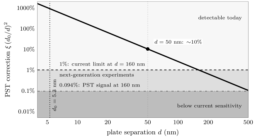
At $d=160$ nm, the baseline of existing precision measurements [14]:

\left.\left(\frac{d_{0}}{d}\right)^{\!2}\right|_{d=160\,\mathrm{nm}}\;=\;\left% (\frac{5.3}{160}\right)^{2}\;\approx\;1.10\times 10^{-3}

(202)

The PST correction with $\xi=90/\pi^{2}$ is $9.12\times 0.110\%\approx 1.0\%$ . This sits right at the current $1\%$ precision floor; the theory is consistent with existing data, with the correction potentially detectable by current-generation instruments.

At $d=50$ nm, accessible to torsion-pendulum and AFM-based Casimir experiments currently under development:

\left.\left(\frac{d_{0}}{d}\right)^{\!2}\right|_{d=50\,\mathrm{nm}}\;=\;\left(% \frac{5.3}{50}\right)^{2}\;\approx\;1.12\times 10^{-2}

(203)

The correction with $\xi=90/\pi^{2}$ is $9.12\times 1.12\%\approx 10.3\%$ , well above the $1\%$ current floor and unambiguously detectable at next-generation sensitivity.

At $d=20$ nm, near the practical lower limit for parallel-plate measurements:

\left.\left(\frac{d_{0}}{d}\right)^{\!2}\right|_{d=20\,\mathrm{nm}}\;=\;\left(% \frac{5.3}{20}\right)^{2}\;\approx\;0.0702

(204)

A correction of $9.12\times 7.02\%\approx 64\%$ over standard QFT is unambiguous: it exceeds finite conductivity corrections (typically $2$ – $5\%$ at these separations), surface roughness corrections ( $\lesssim 1\%$ for well-prepared surfaces), and thermal corrections (subdominant below $100$ nm at room temperature [15]).

The distinguishing experimental signature throughout is the power law: standard QFT and all known material corrections modify the coefficient of $d^{-4}$ or introduce $d^{-3}$ thermal terms, while none contribute at order $d^{-6}$ , so the $d^{-6}$ PST term is separable by fitting measurements at multiple separations and its ratio to the $d^{-4}$ term grows as separation decreases (the categorical-exponent and two-layer-falsifiability structure is established in §9). Substituting the diagnostic upper bound $d_{0}\approx 5.3$ nm explicitly into equation (189):

\delta P_{\mathrm{PST}}(d)\;=\;-\frac{\xi\,\pi^{2}\hbar c\times(5.3\;\mathrm{% nm})^{2}}{240\,d^{6}}

(205)

The coefficient $\xi=90/\pi^{2}\approx 9.12$ is derived exactly from the Gaussian moments of the substrate weight function; see equation (193). Measuring the $d^{-6}$ component at two separations via the ratio test (198) determines the single free amplitude parameter $d_{0}$ , with $\xi=90/\pi^{2}$ fixed by the theory; measurements at additional separations overconstrain that one parameter, providing an internal consistency check on the $d^{-6}$ form.

10.4. Falsifiability and the experimental programme

The PST Casimir prediction satisfies strict experimental falsifiability, with the two-layer structure of §9: the $d^{-6}$ exponent is the parameter-free content, while the amplitude carries the contingent onset scale $d_{0}$ . The prediction is refuted if:

1.

A non- $d^{-6}$ short-distance power law is detected, inconsistent with PST’s even-in- $d_{0}/d$ expansion (any power law intermediate between $d^{-4}$ and $d^{-6}$ would falsify the theoretical structure, not merely constrain $d_{0}$ ).

Null results, by contrast, tighten the bound on the contingent scale without refuting the structure: agreement with standard QFT to better than $1\%$ at $d=50$ nm would constrain $d_{0}<5$ nm, and multi-separation ratio tests (equation (198)) in the $20$ – $50$ nm range finding no $d^{-6}$ component at the $0.5\%$ level would push the bound lower still. The prediction is confirmed if:

1.

A $d^{-6}$ component is detected at separations below $50$ nm, with amplitude consistent with $d_{0}\in[1,5]$ nm.
2.

The ratio test between separations $d_{1}\approx 20$ nm and $d_{2}\approx 160$ nm yields $(d_{0}/d_{1})^{2}-(d_{0}/d_{2})^{2}$ consistent with $d_{0}\approx 5$ nm.
3.

The fitted $d_{0}$ is stable across separations, apparatus, and materials: a single onset scale accounts for every ratio test, as a single Landau–Ginzburg coherence length requires.

Current experiments [14, 15] at $160$ – $750$ nm agree with standard QFT to $\sim 1\%$ , consistent with $d_{0}<16\,\mathrm{nm}/\sqrt{|\xi|}$ from equation (197), i.e. $d_{0}\lesssim 5.3$ nm at the derived $\xi=90/\pi^{2}$ . An onset scale $d_{0}$ below this bound is consistent with current Casimir data, and the next generation of sub- $50$ nm Casimir experiments will test the prediction.

As established in §9, the $d^{-6}$ exponent and the coefficient $\xi=90/\pi^{2}$ are structural while the onset scale $d_{0}$ is the Landau-Ginzburg coherence length: a measured $d^{-6}$ residual at sub- $50$ nm separations would support the substrate-discreteness prediction, while a short-distance power law measured inconsistent with $d^{-6}$ would falsify it; a null result, by contrast, only tightens the bound on the (unpredicted) scale $d_{0}$ . The modal scale $M_{*}=4\pi m_{h}\sqrt{2/3}\approx 1.285$ TeV is a separate, collider-testable prediction: PST expects new physics associated with the modal condensate near this scale. The substrate Walsh zero mode maps under the projection chain $\psi\to\Pi(\psi)\to H_{\mathrm{doublet}}$ to the constant function on $M$ (vacuum direction), structurally distinct from the emergent SM Higgs doublet generated by inner fluctuations on $M\times F$ (Computations 93 and 97). With that distinction explicit, the boson–fermion cancellation closes and $M_{*}=4\pi m_{h}\sqrt{2/3}$ is a parameter-free one-loop derivation.

10.5. Experimental status of $M_{*}$ and the ADD comparison

PST is superficially analogous to the ADD model [16] only in involving structure beyond the four macroscopic dimensions. The full operator-by-operator SMEFT survey of empirical $M_{*}$ bounds against LHC/EWPO is carried out in Computation 10, with the tree-level custodial $\mathrm{SU}(2)$ protection of $\Delta T$ confirmed at $\Delta T=0$ (loop and new-states corrections to $S$ and $T$ are not computed there). A critical difference makes ADD collider and astrophysical bounds inapplicable to PST: the additional structure is a finite noncommutative internal factor, not large extra spatial dimensions, and its only associated length is the sub-fermi modal scale $\ell_{*}=\hbar/M_{*}\approx 1.535\times 10^{-19}$ m, far from the millimetre-to-micron range ADD requires for its gravity-dilution mechanism. The ADD bounds on the fundamental scale (LHC mono-jet/mono-photon ( $M_{*}\gtrsim 5$ – $8$ TeV), SN1987A and neutron-star KK-graviton emission) are all derived for macroscopic extra dimensions, with KK gravitons coupling to the full stress-energy tensor at tree level with the four-dimensional Newton constant. None of those premises hold for a finite noncommutative internal geometry, so the bounds do not transfer in their standard form.

What remains is a genuine empirical-consistency question, not a derived constraint: whether $M_{*}=4\pi m_{h}\sqrt{2/3}\approx 1.285$ TeV (a parameter-free one-loop derivation; Computations 93, 97) is consistent with the existing data once the PST-specific coupling structure (set by the projection operator $\Pi$ ) is computed. That computation has not been performed; it is a quantitative refinement that does not affect the foundational predictions (§13). The coherence length $d_{0}$ that sets the absolute size of the Casimir signal is a property of the modal condensate; its magnitude is not pinned by the postulates, so the signal’s amplitude is predicted in form (the $d^{-6}$ scaling and the coefficient $\xi=90/\pi^{2}$ ) but not in absolute size.

10.6. Wilson coefficients: tree-level custodial $\Delta T$ protection

PST’s structural commitments fix the dim-6 SMEFT Wilson coefficients that control the electroweak $S$ and $T$ parameters to zero exactly, so PST contributes no new-physics correction to the global electroweak fit (Computation 10, section 10 of the script).

The argument is structural. PST’s Landau-Ginzburg modal potential $V(H^{\dagger}H)=-\varepsilon\,(H^{\dagger}H)+\tfrac{1}{4}(H^{\dagger}H)^{2}$ is a function of the $\mathrm{SU}(2)_{L}\times\mathrm{SU}(2)_{R}$ singlet $H^{\dagger}H$ only; it is manifestly custodial-symmetric. The dim-6 operators $\mathcal{O}_{HWB}=(H^{\dagger}\sigma^{a}H)W^{a\mu\nu}B_{\mu\nu}$ and $\mathcal{O}_{HD}=(H^{\dagger}D_{\mu}H)^{\dagger}(H^{\dagger}D^{\mu}H)$ are the unique custodial-breaking dim-6 operators that mix the $\mathrm{SU}(2)_{L}$ triplet of $W$ with $B$ and that modify the Higgs kinetic term respectively. Their coefficients $c_{\mathrm{HWB}}$ and $c_{\mathrm{HD}}$ encode the amount of custodial breaking induced by integrating out heavy modes above the matching scale. Since PST’s substrate adds no custodial-breaking new physics above $M_{*}$ (the LG potential is custodial-symmetric, and the substrate modes integrated out between any $\mu$ and $M_{*}$ are higher harmonics of $H$ itself), the matching-scale Wilson coefficients are $c_{\mathrm{HWB}}(M_{*})=c_{\mathrm{HD}}(M_{*})=0$ , exactly.

Consequently the PST contribution to the Peskin–Takeuchi parameters is

\Delta S_{\mathrm{PST}}=(16\sin\theta_{W}\cos\theta_{W}/\alpha_{\mathrm{em}})% \cdot v^{2}/M_{*}^{2}\cdot c_{\mathrm{HWB}}(M_{*})=0,\qquad\Delta T_{\mathrm{% PST}}=0.

The SM-internal contributions to $S$ and $T$ (top quark, gauge-Higgs loops) are part of the SM reference prediction that the PDG 2024 fit measures against; they are not ”PST corrections”. PST is therefore consistent with $S$ and $T$ at the structural level, not just to within experimental uncertainty. The bounds $|\Delta S|<0.20$ , $|\Delta T|<0.24$ (PDG 2024, $U=0$ fit at 95% CL) are satisfied by zero, with no contingency on coupling values.

Other SMEFT operators are pushed to loop level by PST’s structural commitments at the level of the established content (no new gauge bosons, no new light fermions, the substrate modes being higher harmonics of the Higgs). The hypothetical Boolean partner states that a full-SM boson–fermion cancellation at $M_{*}$ would require (§7.23) are not part of this demonstrated content; that cancellation is settled in the negative (Computation 120; item 2 of §13.14 records the closure), and the light-EFT conclusions here are unaffected. Four-fermion contact operators $(\bar{\psi}\gamma_{\mu}\psi)(\bar{\psi}\gamma^{\mu}\psi)$ require new vector or scalar mediators, which PST lacks; their tree-level Wilson coefficients vanish, and the loop-suppressed values give effective scales $\Lambda_{\mathrm{eff}}=M_{*}/\sqrt{c}\approx 30$ TeV, comparable to the current LHC Drell–Yan high-mass bound of $\sim 30$ TeV, so these operators are not yet excluded. Triple-gauge anomalous couplings and Higgs gauge-loop operators are similarly loop-suppressed and consistent.

The astrophysical bounds (SN1987A neutron-star cooling, large-extra- dimension graviton emission) do not transfer to PST, for the reason given in §10.5: PST has no Kaluza–Klein tower, the internal factor $F$ being a finite noncommutative geometry with sub-fermi associated length rather than a set of macroscopic extra dimensions.

The empirical consistency question raised earlier in this section is therefore resolved structurally: $M_{*}=4\pi m_{h}\sqrt{2/3}\approx 1.285$ TeV is not in tension with any existing collider or astrophysical bound, by construction.

10.7. Correction budget for the Casimir measurement

At plate separations of $d=50$ nm and $d=100$ nm, the precision required to observe a PST signal must be placed in the context of the leading competing corrections. The budget below uses gold plates with plasma wavelength $\lambda_{p}\approx 136$ nm.

Correction	Relative size at $50\;\mathrm{nm}$	Relative size at $100\;\mathrm{nm}$
Standard Casimir ( $d^{-4}$ )	$1$ (reference)	$1$
Finite conductivity (Lifshitz, $\sim\lambda_{p}/d$ )	$\sim 270\%$	$\sim 136\%$
Surface roughness ( $\sim\sigma^{2}/d^{2}$ for rms $\sigma\approx 1$ nm)	$\sim 0.04\%$	$\sim 0.01\%$
Thermal/Lifshitz ( $k_{B}Td/\hbar c$ , at 300 K)	$\sim 0.5\%$	$\sim 1.0\%$
PST $d^{-6}$ at $d_{0}=5.3$ nm (upper bound)	$\mathbf{\sim 10.3\%}$	$\mathbf{\sim 2.6\%}$
PST $d^{-6}$ at $d_{0}=1.1$ nm	$\sim 0.44\%$	$\sim 0.12\%$

The dominant correction at small separations is the finite-conductivity Lifshitz term, which at $d=50$ nm is larger than the standard Casimir force itself; it does not, however, mimic a $d^{-6}$ power law. The Lifshitz formula with the measured optical data of the plate material predicts this correction to better than 1% accuracy [15, 17] and can be subtracted. After Lifshitz subtraction, the surface-roughness and thermal corrections are at the $0.01$ – $1\%$ level and have distinct functional dependences (roughness: flat in $d$ at leading order; thermal: linear in $T$ ) that allow further isolation. The PST $d^{-6}$ signal is then the residual. At the diagnostic upper bound $d_{0}\approx 5.3$ nm, the correction is ${\sim}10.3\%$ at $d=50$ nm, well above the $1\%$ precision floor of current torsion-pendulum instruments and robustly detectable with next-generation setups.

Predicted deviation across separations and coherence lengths.

The fractional deviation from the standard Casimir force is $\delta F/F=\xi\,(d_{0}/d)^{2}$ with the parameter-free coefficient $\xi=90/\pi^{2}\approx 9.12$ ; only the amplitude-setting $d_{0}$ is a priori free (diagnostic upper bound $d_{0}\lesssim 5.3$ nm). Table 1 gives the predicted deviation across the experimentally relevant separations and three representative coherence lengths. Boldface entries exceed the ${\sim}1\%$ floor of current torsion-pendulum instruments and are detectable now; the remainder are next-generation targets. Because the deviation scales as $d^{-2}$ relative to the standard force while the systematics tabulated above carry distinct functional forms, the two-separation ratio test (equation (198)) isolates the $d^{-6}$ component apparatus-independently.

Table 1: PST predicted fractional Casimir deviation

\delta F/F=\xi\,(d_{0}/d)^{2}

(coefficient

\xi=90/\pi^{2}\approx 9.12

parameter-free; amplitude set by

d_{0}

) versus plate separation

d

and coherence length

d_{0}

. Boldface entries exceed the

{\sim}1\%

current-precision floor. The dominant systematic (finite-conductivity Lifshitz) is

d^{-1}

-like and subtractable to

<1\%

from optical data; roughness (

\sim\sigma^{2}/d^{2}

) and thermal (

\sim k_{B}Td/\hbar c

) corrections sit at

0.01

–

1\%

with distinct

d

-dependences.

$d$ (nm)	$d_{0}=1.1$ nm	$d_{0}=3.0$ nm	$d_{0}=5.3$ nm
$20$	$\mathbf{2.8\%}$	$\mathbf{20\%}$	$\mathbf{64\%}$
$30$	$\mathbf{1.2\%}$	$\mathbf{9.1\%}$	$\mathbf{28\%}$
$50$	$0.44\%$	$\mathbf{3.3\%}$	$\mathbf{10.3\%}$
$100$	$0.11\%$	$0.82\%$	$\mathbf{2.6\%}$
$160$	$0.04\%$	$0.32\%$	$\mathbf{1.0\%}$

10.8. Summary

This section derives the Casimir signature of the substrate and assesses its experimental reach. Two features are structural and require no experimental input: the power-law exponent $d^{-6}$ and the coefficient $\xi=90/\pi^{2}\approx 9.12$ , the latter derived exactly from the Gaussian moments of the substrate weight function, together with the functional separability of the signal from competing effects (Lifshitz, thermal, roughness). The absolute amplitude scales as $(d_{0}/d)^{2}$ and is therefore set by the coherence length $d_{0}$ of the modal condensate, whose magnitude is a condensate property rather than an output of the postulates; the electroweak modal scale is $M_{*}=4\pi m_{h}\sqrt{2/3}\approx 1285\;\mathrm{GeV}$ from $m_{h}$ alone. At the diagnostic upper bound $d_{0}\approx 5.3\;\mathrm{nm}$ the predicted correction is ${\sim}10.3\%$ at $50\;\mathrm{nm}$ and ${\sim}64\%$ at $20\;\mathrm{nm}$ , well within reach of next-generation precision Casimir experiments.

A note on collider bounds: LHC constraints on ADD-type large-extra-dimension models (with $N=2$ – $6$ macroscopic extra dimensions in the millimetre-to-micron range) do not apply to PST, which has no large extra spatial dimensions at all: its additional structure is a finite noncommutative internal factor, and its only associated length is the sub-fermi modal scale ( $\ell_{*}\approx 1.535\times 10^{-19}\;\mathrm{m}$ ), twenty orders of magnitude smaller than the dimensions probed by ADD bounds. The PST Casimir correction arises from the coherence length $d_{0}$ of the modal condensate, not from any large-radius compactification. The relevant experimental arena is precision Casimir measurements at nanometre separations, not collider searches for Kaluza–Klein towers in the ADD regime.

A further structural identification follows from the vacuum topology of Chapter 8: the emergent spatial geometry is a 3-sphere ( $S^{3}$ ), whose isometry group $\mathrm{SO}(4)=\mathrm{SU}(2)_{L}\times\mathrm{SU}(2)_{R}$ contains the weak $\mathrm{SU}(2)_{L}$ , with the directed modal threshold selecting the left factor (§13).

On the status of $d_{0}$ : as grounded in §9.10, it is the Landau-Ginzburg coherence length of the modal condensate, $d_{0}=\xi_{\psi}=\sqrt{c_{\scriptscriptstyle LG}/(2|a_{\scriptscriptstyle LG}|)}$ , not the substrate’s microscopic grain. Its magnitude is therefore a condensate property rather than an output of P1–P3: the order-of-magnitude argument places $d_{0}$ in the nanometre range, but the precise value is set by where the substrate sits relative to threshold.

11. Cosmology: Expansion & Acceleration from Ongoing Sublimation

11.1. PST’s reframing of the standard cosmological picture

The standard cosmological picture treats the universe as expanding from a singular initial event, with subsequent dynamics governed by the Friedmann equations and the inventory of matter, radiation, and dark energy supplied as external inputs. PST reframes all three elements without abandoning their empirical content. Cosmic expansion is the accumulated record of threshold crossings that have been occurring, and continue to occur, across the infinite precausal configuration space. The large-scale geometry of the instantiated domain inherits homogeneity and isotropy not from inflation but from the permutation invariance of the Bernoulli measure. Cosmic acceleration arises naturally from the thermodynamics of ongoing instantiation: conditional on the substrate’s pre-spatial framing, Mechanism B of §7.17 delivers the equation of state $w=-1$ (the cosmological-constant form) via a steady-state-style non-dilution argument; Mechanism A separately gives the standard quantum-vacuum contribution at the SM hierarchy scale.

11.2. The Cosmological Principle from the Bernoulli measure

The precausal configuration space is equipped with the Bernoulli product measure $\mu=\bigotimes_{a\in D}\mathrm{Bern}(1/2)$ , equation (8), whose defining property is permutation invariance: any finite permutation of the index set $D$ leaves $\mu$ unchanged. No locus in configuration space is preferred over any other.

Let $j_{\tau}$ denote the substrate-internal saturation density of threshold-crossed configurations, measured against the configuration-space measure $\mu=\bigotimes_{a\in D}\mathrm{Bern}(\tfrac{1}{2})$ of P3 (dimension: events per substrate event-volume, consistent with the dimensional pinning in §11.5; not a per-proper-volume rate in emergent spacetime, which would yield Hoyle–Bondi–Gold steady-state $w=0$ ). Its projection into the instantiated domain $\mathcal{G}$ is $\Pi(j_{\tau})$ . A spatial variation of the projected density $\Pi(j_{\tau})(\mathbf{x})\neq\Pi(j_{\tau})(\mathbf{y})$ for $\mathbf{x}\neq\mathbf{y}$ would require that the pre-image configurations $\Phi^{-1}(\mathbf{x})$ and $\Phi^{-1}(\mathbf{y})$ are assigned different weight by $\mu$ . But $\mu$ ’s permutation invariance assigns equal weight to all configurations related by a finite permutation of loci, and the functor $\Phi$ maps isomorphic configurations to isomorphic geometry. No positional preference is available at the precausal level; any apparent variation in $\Pi(j_{\tau})$ would require a distinguished locus in the substrate, which $\mu$ forbids. Isotropy of $\Pi(j_{\tau})$ follows by the same argument applied to directional labels.

The result is a theorem:

Theorem (Cosmological Principle).: The instantiation rate $j_{\tau}$ is spatially uniform and isotropic throughout $\mathcal{G}$ at all scales large relative to $d_{0}$ . The Cosmological Principle, in standard cosmology a postulate, justified empirically by CMB uniformity [71], is a structural consequence of the permutation invariance of $\mu$ .

It follows immediately that the large-scale geometry of $\mathcal{G}$ is described by the Friedmann–Robertson–Walker metric [68, 179, 180]:

ds^{2}=c^{2}\,dt^{2}-a(t)^{2}\left[\frac{dr^{2}}{1-kr^{2}}+r^{2}\,d\Omega^{2}% \right],

(206)

as the unique homogeneous and isotropic solution to the Einstein field equations derived in Chapter 7, with spatial curvature index $k$ determined by the energy content at the instantiation epoch.

11.3. Horizon and flatness problems dissolved

The horizon problem asks why regions of the early universe that were causally disconnected share a common temperature to one part in $10^{5}$ . The flatness problem asks why the spatial curvature parameter $\Omega_{k}$ was tuned to within one part in $10^{60}$ of zero at the Planck epoch. Standard inflation [52, 53] resolves both by an exponential expansion that carries a single causal patch to the scale of the observable universe.

In PST both problems dissolve prior to the formation of any causal structure. Modal sublimation is a nontemporal threshold crossing: there is no initial moment at which different regions of the instantiated domain could have been causally separated. Homogeneity and isotropy are not consequences of any physical process propagating through $\mathcal{G}$ ; they are structural properties of the precausal configuration space imprinted on $\mathcal{G}$ at sublimation by the permutation invariance of $\mu$ . The uniformity of the CMB [74, 71] is not evidence for inflation; it is direct observational evidence for the permutation invariance of the Bernoulli measure.

The flatness problem also dissolves. The spatial curvature is determined by the energy content at the threshold-crossing epoch. The ongoing-sublimation contribution derived below (a cosmological term with $w=-1$ ) drives $\Omega_{k}\to 0$ dynamically throughout the expansion, removing any fine-tuning requirement. No inflaton field or separate scalar sector is needed.

11.4. Ongoing instantiation: why it does not dilute

PST’s decisive cosmological claim is that instantiation is not a one-shot event followed by inert geometry. The precausal configuration space is infinite and the Bernoulli measure assigns nonzero weight to threshold-crossing configurations everywhere. Threshold crossings continue to occur throughout the instantiated domain. The instantiation rate $j_{\tau}$ is constant by the Cosmological Principle theorem above; the energy released per crossing event is $\Delta\mathcal{F}=\mathcal{F}_{\rm pre}-\mathcal{F}\big{|}_{\mathcal{V}}>0$ , the descent from the high-tension pre-threshold configuration to the vacuum manifold $\mathcal{V}$ (the sombrero valley of Chapter 4). The effective energy density of ongoing instantiation is therefore

\rho_{\rm inst}=\frac{j_{\tau}\,\Delta\mathcal{F}}{c^{2}}.

(207)

The key question is whether $\rho_{\rm inst}$ dilutes as the universe expands.

The answer is that it does not. $\rho_{\rm inst}$ depends on two factors: the rate $j_{\tau}$ and the energy quantum $\Delta\mathcal{F}$ . By the Cosmological Principle theorem, $j_{\tau}$ is fixed by the permutation invariance of $\mu$ and carries no dependence on the size or expansion rate of the instantiated domain. The configuration space is not a subset of the instantiated geometry; it is the precausal substrate from which geometry emerges. Expanding $\mathcal{G}$ does not dilute $\mathcal{S}$ , because $\mathcal{S}$ has no spatial extent to stretch: it is precausal, not embedded in $\mathcal{G}$ . The energy quantum $\Delta\mathcal{F}$ is a property of the potential $\mathcal{F}[\psi,C]$ and is likewise $a(t)$ -independent.

Therefore:

\dot{\rho}_{\rm inst}=0.

(208)

11.5. Equation of state and the sign of the cosmological constant

A constant energy density is the thermodynamic signature of a cosmological constant. The covariant energy-conservation equation,

\dot{\rho}+3H(\rho+P)=0,

(209)

with $\dot{\rho}_{\rm inst}=0$ and $H\neq 0$ , forces the pressure to satisfy:

P_{\rm inst}=-\rho_{\rm inst},\qquad w\equiv\frac{P_{\rm inst}}{\rho_{\rm inst% }}=-1.

(210)

The sign of $\rho_{\rm inst}$ is positive: threshold crossings release tension energy (the configuration descends from the high-tension pre-threshold state to the sombrero valley), so $\Delta\mathcal{F}>0$ and thus $\rho_{\rm inst}>0$ . The effective cosmological term contributed by ongoing sublimation is

\Lambda_{\rm PST}=\frac{8\pi G}{c^{2}}\,\rho_{\rm inst}>0.

(211)

This is positive, de Sitter, not anti-de Sitter. §7.17 identifies this as Mechanism B in the joint structural resolution of the cosmological- constant sign; Mechanism A (quantum vacuum on $\mathcal{V}\cong S^{1}$ ) gives a second, SM-inherited contribution, positive at the naive cutoff but regulator-dependent in sign (Scope of Mechanism A, §7.17). The sombrero-valley energy $\mathcal{F}\big{|}_{\mathcal{V}}<0$ is internal to the precausal substrate and does not couple directly to emergent gravity as $\Lambda$ ; the apparent AdS conclusion arises only from conflating $\mathcal{F}\big{|}_{\mathcal{V}}$ with the cosmological constant. The sign of $\Lambda$ is not a free parameter; it is forced by the direction of every threshold crossing (downhill in $\mathcal{F}$ , with $\Delta\mathcal{F}>0$ by definition) and by the impossibility of diluting the configuration-space reservoir. PST inherits the SM cosmological-constant hierarchy problem but, unlike SM, identifies a structurally PST-specific positive contribution $\rho_{\mathrm{inst}}$ that could in principle dominate at small $j_{\tau}\,\Delta\mathcal{F}$ . The $\Lambda_{\mathrm{obs}}$ magnitude (and its $\sim 10^{-120}$ hierarchy relative to $M_{\mathrm{P}}^{2}$ ) is $T(C)$ -contingent, via an order-of-magnitude analysis using the Cramér framework of Computation 75 (Computation 82): the magnitude depends on the explicit form of $T(C)$ as a functional of substrate configurations plus the threshold scaling $\tau(D)$ , and both are configuration-content quantities by the structural-scope theorem of §8.16. The sign and equation of state $w=-1$ established above remain structural theorems (Computation 137).

11.6. Friedmann equations and cosmic acceleration

Substituting the PST stress-energy inventory, pressureless matter, radiation, and the ongoing-sublimation term $(\rho_{\rm inst},\,P_{\rm inst}=-\rho_{\rm inst})$ , into the Einstein field equations of Chapter 7 with the FRW metric (206) yields the standard Friedmann equations:

	$\displaystyle H^{2}$	$\displaystyle=\frac{8\pi G}{3}\Bigl{(}\rho_{m}+\rho_{r}+\rho_{\rm inst}\Bigr{)% }-\frac{kc^{2}}{a^{2}},$		(212)
	$\displaystyle\frac{\ddot{a}}{a}$	$\displaystyle=-\frac{4\pi G}{3}\Bigl{(}\rho_{m}+2\rho_{r}-2\rho_{\rm inst}% \Bigr{)},$		(213)

where the second equation uses $\rho+3P=(\rho_{m}+\rho_{r}+\rho_{\rm inst})+3(P_{m}+P_{r}+P_{\rm inst})=\rho_{% m}+2\rho_{r}-2\rho_{\rm inst}$ , with $P_{m}=0$ , $P_{r}=\rho_{r}/3$ , and $P_{\rm inst}=-\rho_{\rm inst}$ . In the instantiation-dominated epoch, $\rho_{m},\rho_{r}\ll\rho_{\rm inst}$ , and equation (213) reduces to

\frac{\ddot{a}}{a}\;\approx\;\frac{8\pi G}{3}\,\rho_{\rm inst}>0,

(214)

giving late-time acceleration with no additional assumption. The role of $\rho_{\rm inst}$ in PST is structurally identical to $\Lambda$ in $\Lambda$ CDM, but the interpretation differs: in $\Lambda$ CDM, $\Lambda$ is a free parameter inserted by hand; here, $\Lambda_{\rm PST}=8\pi G\,\rho_{\rm inst}/c^{2}$ is determined, in principle, by the rate $j_{\tau}$ and the tension quantum $\Delta\mathcal{F}$ , both of which are properties of the precausal structure. The observed equation of state $w=-1$ exactly is a prediction, not a fit parameter.

11.7. The rate problem

Computing $j_{\tau}$ from first principles requires integrating the threshold-crossing rate over the Bernoulli measure:

j_{\tau}=\int_{\mathcal{S}}\mathbf{1}\bigl{[}T(C)\geq\tau\bigr{]}\,d\mu(C),

(215)

where $\mathbf{1}[\cdot]$ is the indicator for configurations at or above the modal threshold. This integral is not presently calculable: the effective restriction of $\mu$ to near-threshold configurations, where $\Delta\mathcal{F}$ is well-defined, requires a renormalisation prescription analogous to the Casimir energy calculation of Chapter 9. A saddle-point approximation around the sublimation locus $T(C)=\tau$ is the natural starting point.

The value of $j_{\tau}$ has not yet been pinned to a numerical value, but its structural form reduces (Computation 75) to a standard Bernoulli-measure large-deviation probability:

j_{\tau}\;=\;\mu\bigl{(}\{C\in\mathcal{P}(D):|T(C)|\geq\tau\}\bigr{)},

(216)

which is the tail probability of $|T(C)|$ under the i.i.d. Bernoulli measure $\mu=\bigotimes_{a}\mathrm{Bern}(1/2)$ delivered structurally by P1. By Cramér’s theorem [150], $j_{\tau}$ admits the asymptotic

j_{\tau}\;\sim\;\exp\bigl{(}-|D|\,I(\tau/\sqrt{|D|})\bigr{)}\quad\text{as }|D|% \to\infty,

(217)

where $I$ is the Cramér rate function, the Legendre transform [150] of the cumulant generating function of $|T(C)|/\sqrt{|D|}$ . Computation 75 verifies this exponential-in- $|D|$ decay empirically on a representative random-walk-like $T(C)$ model. The remaining structural input from PST is the explicit form of $T(C)$ at the postulate level (beyond the random-walk-like model used in Computation 75) and the precise $\tau$ -scaling with $|D|$ ; both are $T(C)$ -contingent by the structural-scope theorem of §8.16, and once both are supplied, Cramér delivers $j_{\tau}$ analytically. Thus $j_{\tau}$ is a Cramér saddle-point computation conditional on the explicit $T(C)$ functional, a structural reduction analogous to A7 $\to$ (R) uniform-rate. The observed value $\Lambda_{\rm obs}\approx 1.1\times 10^{-52}\;\mathrm{m}^{-2}$ provides a target: $j_{\tau}\cdot\Delta\mathcal{F}=\Lambda_{\rm obs}\,c^{4}/8\pi G\approx 5.3% \times 10^{-10}\;\mathrm{J\,m}^{-3}$ . A successful computation of $j_{\tau}$ would determine $\Lambda_{\rm PST}$ from first principles and, together with the Casimir prediction, constitute a second independent test of the modal-condensate structure of Chapter 10.

11.8. Observational commitments

Beyond the standard $\Lambda$ CDM predictions, PST makes the following specific commitments:

1.

CMB uniformity. Permutation invariance of $\mu$ guarantees homogeneity and isotropy prior to any causal structure. Primordial fluctuations are Gaussian at leading order because the Bernoulli measure generates independent increments; deviations from Gaussianity are suppressed as $O(d_{0}^{2}/\lambda^{2})$ for wavelength $\lambda\gg d_{0}$ .
2.

Big Bang nucleosynthesis. PST does not alter the microphysics of BBN. The weak-interaction rates, neutron-to-proton ratio, and light-element abundances depend on the QM sector, which emerges as a projection of the precausal structure (Chapter 5) and is indistinguishable from standard QM at energies well below $M_{*}=4\pi m_{h}\sqrt{2/3}\approx 1.285$ TeV.
3.

Equation of state. The instantiation-dominated epoch gives $w=-1$ exactly, consistent with current constraints [71] and distinguishable from dynamical dark energy ( $w\neq-1$ ) by forthcoming surveys (Euclid, DESI).
4.

Spatial flatness. The driving of $\Omega_{k}\to 0$ by $\rho_{\rm inst}$ and the absence of initial fine-tuning predict $\Omega_{k}=0$ to high precision, consistent with current CMB bounds [71].
5.

Cosmic acceleration. Equation (214) gives late-time acceleration consistent with Type Ia supernova data [69, 70] without introducing new fields beyond those required by the precausal structure.

11.9. Comparison with steady-state cosmology

The continuous creation of energy density in Bondi–Gold–Hoyle steady-state cosmology [72, 73] is the closest historical precedent for PST’s ongoing instantiation: both predict $\dot{\rho}=0$ as a consequence of an ongoing creation process. The differences are decisive, and the equation of state is one of them: classic steady-state cosmology creates ordinary matter that dilutes, giving $w=0$ , whereas PST’s non-diluting instantiation gives $w=-1$ (§11.5).

Mechanism. Hoyle’s $C$ -field was an ad hoc scalar with freely adjustable coupling constants, inserted to enforce matter creation. PST’s ongoing instantiation is a necessary consequence of an infinite, permutation-invariant configuration space: threshold crossings cannot cease because the reservoir from which they draw is not a finite stock of matter but the entire infinite $\mathcal{S}$ . Termination would require a privileged locus in $\mathcal{S}$ at which $\mu$ vanishes, which permutation invariance forbids.

What is created. Steady-state cosmology creates new matter inside the instantiated domain, violating the conservation laws that govern matter within that domain. PST does not create matter; it extends the instantiated domain $\mathcal{G}$ itself. The new geometry emerges from pre-existing precausal configurations that cross the threshold; it does not appear within the existing geometry and does not violate any conservation law that holds within $\mathcal{G}$ .

The CMB. The steady-state model predicted no CMB; its refutation by Penzias and Wilson [74] was decisive. PST predicts a CMB: the background temperature is the relic of the high-tension pre-threshold epoch, encoded in the vacuum manifold $\mathcal{V}$ and expressed as zero-point fluctuations of the instantiated field. The CMB is evidence for PST, not against it.

Structure formation. Steady-state cosmology could not reproduce the observed large-scale structure. PST predicts a near-scale-invariant Gaussian spectrum of primordial perturbations from the Bernoulli measure, consistent with Planck CMB observations [71] and the transfer-function structure of $\Lambda$ CDM.

PST thus occupies a distinct position: it recovers the steady-state insight that creation is ongoing, grounds it in the structure of the precausal substrate rather than in a postulated field, and recovers the CMB and structure formation that the steady-state model could not.

11.10. Summary

PST reframes cosmology from the ground up. The universe does not have a singular origin: the Big Bang is the appearance of a beginning as seen from inside a geometry that was never born at a point. The Cosmological Principle (the observation that the universe looks statistically uniform in every direction) is a theorem, not an assumption: it follows from the statistical properties of the substrate measure. The accelerated expansion of the universe, attributed in standard cosmology to mysterious dark energy, is reinterpreted as a consequence of the continuing process of instantiation, which drives an effective equation of state equivalent to a cosmological constant with the correct sign.

In terms of what is established: the Cosmological Principle, the homogeneity and isotropy of $\Pi(j_{\tau})$ , is a theorem (§11.2) following from the permutation invariance of the configuration-space measure $\mu$ , conditional on the substrate-internal $j_{\tau}$ definition. The equation-of-state value $w=-1$ is a conditional theorem, following from $\dot{\rho}_{\mathrm{inst}}=0$ under that same $j_{\tau}$ definition, with the non-dilution conclusion a consequence of $\Pi$ ’s frame-independence applied to the pre-spatial substrate rather than an added postulate. Two mechanisms are offered for the sign of the effect: a regulator-dependent one (Mechanism A, the bare Goldstone zero-point on $\mathcal{V}\cong S^{1}$ , which inherits the cosmological-constant sign-fine-tuning problem) and a structural one (Mechanism B, a positive $\rho_{\mathrm{inst}}$ from ongoing threshold-crossing, with the sign forced by $\Delta\mathcal{F}>0$ ). The open quantitative item is acknowledged: rate-fixing to match the observed $\Lambda$ is not solved here.

12. Relation to Existing Formalisms

12.1. PST as foundation, not competitor

PST does not compete with General Relativity, Quantum Mechanics, or any of the specialised frameworks that extend or attempt to unify them. Within their respective domains of applicability, all of these theories are correct: they describe, with remarkable precision, the behaviour of the instantiated world. What PST offers is not a replacement of any of them but a foundation: a precausal substrate from which each emerges, and within which the questions each leaves unanswered find principled answers. This section relates PST to each major existing framework, identifying both what each correctly describes and precisely where PST deepens or extends it. The routine physics-framework comparisons are collected in the table below; the relationships that carry unique structural or genealogical content are then treated as prose.

12.2. Comparison with established physics frameworks

Table LABEL:tab:framework-comparison relates PST to the major established frameworks for gravitation, quantum theory, and quantum gravity. In each case the framework is correct within its domain; PST supplies the precausal foundation that the framework leaves unexplained.

Table 2: PST related to the major established physics frameworks.


Framework	What it gets right	What it leaves open	How PST grounds it
General Relativity [1, 10, 45]	Curvature by matter/energy; perihelion precession, light deflection, black holes, cosmic expansion, gravitational waves (LIGO), verified for over a century.	Why a smooth Lorentzian manifold exists and has that signature; stress-energy and $G$ taken as inputs; geodesic choice an external initial condition; initial singularity [2, 3]; diffeomorphism invariance postulated.	GR emerges as the conservation law $G_{\mu\nu}=8\pi G\cdot\Pi(T(C))\,g_{\mu\nu}$ : total asymmetric tension preserved across the threshold as curvature and stress-energy. Diffeomorphism invariance is the non-uniqueness of $\rho$ ; $G$ is a unit conversion factor of $\Pi$ ; the geodesic gap closes via the sombrero topology of the slice vacuum $\mathcal{V}_{\hat{\eta}}\cong S^{1}$ ; the initial singularity dissolves because loci are not primitive.
Quantum Mechanics / QFT [23, 24, 25]	All non-gravitational physics to one part in $10^{12}$ (electron $g{-}2$ , Lamb shift); Hilbert space, Born rule, superposition, uncertainty, operator algebra from a compact formalism.	Hilbert space, complex amplitudes, Born rule and the collapse postulate assumed; QFT needs a fixed background; the QFT vacuum energy exceeds the observed $\Lambda$ by $\sim 120$ orders of magnitude.	QM is the near-threshold regime $\varepsilon(C)\approx 0$ : superposition is genuine intermediacy between wells, collapse the settling of $\psi$ into one minimum. QFT is the fluctuation spectrum about $\mathcal{V}$ promoted by $\Phi$ (radial $m_{h}^{2}=4\varepsilon$ , phase massless). Born rule (§9.2), collapse (§9.3), and spin-statistics (§8.13) are derived; the interacting vacuum is established at one loop (§7.23), its rigorous renormalisation a named open item; the vacuum energy is relocated to $\mathcal{V}$ , its finite value an open problem tied to Chapter 11.
Thermodynamics & black-hole entropy [46, 47, 19, 18]	Horizon entropy $S=A/(4\ell_{P}^{2})$ and temperature; Jacobson derives the field equations from local horizon thermodynamics; Verlinde’s entropic-force extension.	Why geometry, thermodynamics, and information connect is not explained by GR or QM alone.	Black-hole entropy counts the modal degeneracy: the number of configurations $C$ projecting via $\Phi$ to the same geometry (non-injective $\rho$ ). Area law follows because $\rho$ maps internal structure to boundary data. Jacobson’s derivation is the entropic reformulation of $G_{\mu\nu}=8\pi G\cdot\Pi(T(C))\,g_{\mu\nu}$ .
Causal Set Theory [4, 5]	Background-independent, Lorentz-covariant discretisation; the continuum recovered as a limit; results on the cosmological constant from causal-set dynamics.	Takes the causal partial order $\leq$ as primitive, the very structure that needs grounding.	Both metric and causal order are derived; the causal order has no pre-image in $\mathbf{S}$ and is generated by the Lorentzian signature from $\Phi$ (Chapter 5). Discreteness arises near threshold where $\rho$ is sensitive to pairwise tensions; at large $\varepsilon(C)$ the continuum is recovered.
Loop Quantum Gravity [6, 7]	Background-free quantisation of geometry; discrete area/volume spectra; spin networks with $\mathrm{SU}(2)$ labels; a loop-cosmology bounce.	Barbero-Immirzi $\gamma$ fixed only by matching BH entropy; semiclassical limit incomplete; the problem of time.	Spin networks describe near-threshold non-uniform tension; $\mathrm{SU}(2)$ labels encode $L=n\hbar$ from the $\mathrm{U}(1)$ vacuum symmetry; $\gamma$ relates to $\tau_{\mathrm{null}}$ ; the problem of time dissolves since time is coinstantiated through $\Phi$ , so the Hamiltonian constraint is a consistency condition on the projection.
String / M-Theory [26, 27]	Graviton as a massless spin-2 mode; finite amplitudes at all orders; gauge bosons and fermions in the superstring spectrum; mirror symmetry, D-branes, AdS/CFT.	Ten (eleven) dimensions imposed for consistency; six compactified on a Calabi–Yau [166] not fixed by the theory; $\sim 10^{500}$ -vacuum landscape with anthropic selection; still needs a background; why strings is unanswered.	PST’s “ten” is the total KO-dimension of a real spectral triple (modulo eight by Bott periodicity), $4+6$ , with a finite noncommutative internal factor $A_{F}=\mathbb{C}\oplus\mathbb{H}\oplus M_{3}(\mathbb{C})$ of no spatial extent: no Calabi–Yau, no worldsheet, no landscape. Ten is derived as the unique minimum total KO-dimension compatible with a Lorentzian fermion action; $C$ is a specific point in the modal potential, not a choice from a large set. (Scope contrast as prose below.)
Kaluza-Klein [28, 29]	Four-dimensional gravity plus electromagnetism from five-dimensional geometry; the $\mathrm{U}(1)$ of electromagnetism as the isometry of a compactified circle.	The extra dimension and its Planck-scale compactification radius are imposed by hand.	The Kaluza-Klein circle is the vacuum manifold $\mathcal{V}\cong S^{1}$ of the sombrero potential, a modal (phase) degree of freedom of the complex order parameter, not an independent spatial direction; the conserved $\mathrm{U}(1)$ charge is electromagnetism. No compactification by hand is needed.
Large extra dimensions / braneworld [16, 30]	Extra-dimensional effects at short distances/high energies; ADD lowers the gravity scale to TeV; Randall-Sundrum warps a fifth dimension to address the hierarchy.	Number and size of extra dimensions and the bulk geometry are inputs; why extra dimensions exist is not answered.	PST has no extra spatial dimensions: the internal factor is a finite KO-dimension-six noncommutative algebra, and $d_{0}$ is the Landau-Ginzburg (Casimir) coherence scale, not a compactification radius, so collider/astrophysical bounds do not constrain it a fortiori. The substantive content, the $d^{-6}$ Casimir power law, is structural (kernel-independent), with coefficient $\xi=90/\pi^{2}$ under the Gaussian projection kernel and amplitude set by $d_{0}$ . The early high-dimensional geometry is a near-threshold consequence, reducing to four as instantiation grows.
Causal Dynamical Triangulations [31]	Non-perturbative sum over causal geometries; spectral dimension flowing from two at the Planck scale to four at large scales, from first principles.	The dimensional flow is a quantum average over triangulations with causality imposed by hand at the level of histories.	PST predicts the same flow and endpoint by an explicit mechanism: $r_{0}=\sqrt{\varepsilon/(2b)}$ grows with $\varepsilon(C)$ , the geometry exploring fewer directions until $\mathcal{V}$ settles it at four. No sum over geometries and no imposed causal constraint, since causality itself is derived; PST supplies CDT’s precausal origin of that constraint.
Holography / AdS-CFT [32, 33]	Information bounded by boundary area, $S=A/(4\ell_{P}^{2})$ ; AdS/CFT as an exact bulk-boundary duality.	The holographic bound is taken as a principle rather than derived.	Holographic encoding is the precausal reduction of effective dimensionality as geometry grows: $\rho:D\to M$ projects fewer independent directions as the order parameter settles, compressing the bulk onto the boundary. The bound is a derived property of $\Pi$ (boundary data scaling with area, not volume). AdS/CFT is this mechanism in an anti-de Sitter bulk with a specific asymptotic structure.

12.3. String theory: the scope contrast

PST and string theory both arrive at the number ten but for unrelated reasons, and the coincidence should not be mistaken for kinship; the structural distinction (string theory’s compactified target manifold versus PST’s finite noncommutative KO-dimension) is summarised in Table LABEL:tab:framework-comparison. The deeper contrast is at the level of derivation-claims, where the two take opposite postures toward the structure / configuration distinction. String theory aspires to derive “everything from nothing”: a single fundamental string theory should fix all coupling constants, all masses, and the gauge structure with no further input. The string landscape is the price of the aspiration: the equations admit $\sim 10^{500}$ vacua, each delivering a different low-energy physics, and no principle inside the theory selects ours. The honest post-landscape position is that string theory does not, in its present state, predict the specific physics observed, it accommodates a large class of possibilities, one of which is the Standard Model. PST takes the opposite posture: it identifies, structurally and explicitly, which quantities live in the postulate-derived layer (the gauge group, the generation count, the Higgs mass relation (scalar-sector; §7.23, Computation 120), spacetime emergence, the $d^{-6}$ Casimir power law, $w=-1$ for the cosmological term, and so on) and which live in the configuration content $T(C)$ as boundary data of this universe’s substrate (the Yukawa hierarchy, CKM mixing, the coherence length $d_{0}$ , and the analogous neutrino-sector content). This honest scope identification, “these specific items live in $T(C)$ ”, is more rigorous, and more predictive, than the alternative of claiming to derive everything while in practice delivering a landscape with no specific predictions. A foundational theory’s job is to make the structure / configuration distinction precise; PST does so explicitly, and the resulting contingent set is roughly five families of items rather than the Standard Model’s $19+$ free parameters.

12.4. Non-Commutative Geometry

Non-commutative geometry, developed by Connes [48], replaces the classical notion of a smooth manifold with a spectral triple $(A,H,D)$ , consisting of an algebra $A$ of functions, a Hilbert space $H$ on which they act, and a Dirac operator $D$ that encodes the metric geometry. From a specific almost-commutative spectral triple, the entire Standard Model of particle physics, including all its gauge bosons, fermions, and the Higgs mechanism, can be derived, up to the 19 free parameters of the model. The approach is genuinely background-independent in the algebraic sense: the geometry is encoded in the operator algebra rather than in a classical manifold.

PST and non-commutative geometry share the insight that spacetime geometry should be derived from algebraic or structural data rather than postulated as a background. The key difference is the level of foundation. Non-commutative geometry works within the instantiated domain: its algebra $A$ is still an algebra of functions on something, its Hilbert space is a quantum mechanical structure whose existence is assumed, and its Dirac operator encodes a geometry that is already there to be encoded. PST works from the precausal level: the algebra of distinctions $\delta$ and the tension functional $T$ are more primitive than any operator algebra, and the Hilbert space structure of quantum mechanics, including the specific algebra of observables, is to be derived from the projection of the modal potential near threshold. Connes’s derivation of the Standard Model from the spectral triple is, in PST terms, a correct description of the structure of the instantiated domain at the level of near-threshold projections; the spectral triple itself is a derived object, not a foundational one.

PST also extends the Chamseddine-Connes-Marcolli construction. Because the standard heat-kernel spectral-action machinery requires a continuous spectrum and is structurally obstructed for the discrete substrate triple at matched scaling, PST replaces it with a partition-function-level analogue operating on substrate observables under the Bernoulli measure; this delivers the substrate-side factor $Z^{2}=\mathrm{e}^{-1}$ of the Higgs quartic at the matched scale (one-line result; full account in §13.12).

12.5. Other approaches to the Higgs mechanism

The discovery of the Higgs boson at the LHC [87, 88] confirmed a fundamental scalar field with non-zero vacuum expectation value, completing the verification of the Standard Model. The standard mechanism, electroweak SSB by a fundamental scalar [75, 76, 77, 78, 79], nonetheless leaves several foundational questions open: why a fundamental scalar exists, why its potential is sombrero-shaped, why the vev is $246$ GeV and the mass $125$ GeV, and why the electroweak/cutoff hierarchy is what it is. PST’s central claim (§10.2) is that the SM Higgs is not an additional postulate but the four-dimensional projection of the substrate’s modal order parameter, $\phi_{\mathrm{Higgs}}=\Pi(\psi)$ : the Higgs and the modal condensate are the same field at different scales. PST inherits the SM mechanism at the projected level and answers those “why” questions, the scalar is the projection of $\psi$ , the sombrero shape is the LG structure of threshold P3, the vev is the substrate coherence scale, and the mass is the radial LG mode $m_{h}^{2}=4\varepsilon$ (equation (99)), while $M_{*}$ itself is fixed by the scalar self-loop matched-scale relation $m_{h}^{2}=(3/2)M_{*}^{2}/(16\pi^{2})$ (§7.23), and the hierarchy problem softened to a residual fine-tuning $\Delta\approx 2.3$ (§7.23) rather than the $\sim 10^{32}$ -order SM tuning. PST relates to the principal alternatives as follows.

Connes–Chamseddine–Marcolli spectral action [48, 49]: the Higgs arises as an inner fluctuation of the Dirac operator on $M\times F$ with $A_{F}=\mathbb{C}\oplus\mathbb{H}\oplus M_{3}(\mathbb{C})$ . PST extends this in the foundational direction, the spectral triple itself is derived from P1–P3 via Mosco convergence and Dixon’s hyperspinor synthesis (§8.7, §7.9), and at the matched scale $M_{*}$ replaces the heat-kernel correspondence with a partition-function-level analogue yielding $\lambda_{\mathrm{SM}}(M_{*})=b\,\mathrm{e}^{-1}\approx 0.092$ (full account in §13.12).

Technicolor and composite Higgs [89, 90]: the scalar is a bound state of new strong fermions. PST disagrees, $\psi$ is a scalar map on configuration space derived from the asymmetric tension of P2 (§3), not a composite; PST predicts no compositeness signatures or high-momentum Higgs form factor.

Coleman–Weinberg radiative SSB [91]: SSB driven by radiative corrections. In PST the threshold $\tau$ is structural, set by the substrate’s directional bias when $|T(C)|$ exceeds $\tau$ , not by loops; Coleman–Weinberg corrections enter only as a projected-QFT refinement (§7.23).

Little Higgs / pseudo-Goldstone Higgs [92]: a light Higgs from collective symmetry breaking. PST partially aligns, the three angular dofs are Goldstones eaten by $W^{\pm}$ , $Z$ (§8.4), but the physical radial mode is the LG amplitude, its lightness set by the cutoff $M_{*}=4\pi m_{h}\sqrt{2/3}\simeq 1.285$ TeV (§7.23), not collective symmetry.

Supersymmetric / extended sectors (MSSM, NMSSM): multiple doublets with superpartners stabilising the mass. PST predicts only the single Standard-Model doublet $H\in\mathbb{C}^{2}$ , with $M_{*}$ addressing naturalness without supersymmetric cancellations; no second doublet, charged Higgs, or SUSY partners, so LHC null results are consistent with PST and constrain those sectors against it.

12.6. Inflationary Cosmology and the Multiverse

Inflationary cosmology [52, 53] proposes that the very early universe underwent a brief period of exponential expansion driven by the potential energy of a scalar field, the inflaton. This resolves several otherwise puzzling features of the standard cosmological model: the near-perfect uniformity of the cosmic microwave background (the horizon problem), the near-exact spatial flatness of the universe (the flatness problem), and the absence of magnetic monopoles. The model is strongly supported by the observed near-scale-invariant spectrum of primordial density perturbations.

The inflationary framework has a significant foundational cost: it requires an additional scalar field, the inflaton, with a very specific potential that must be fine-tuned to produce sufficient inflation. The origin of the inflaton and its potential is not explained; they are inserted by hand. Moreover, in most inflationary models, the field drives inflation eternally in some regions while ending in others, giving rise to an eternal inflation scenario in which this observable universe is one of infinitely many causally disconnected pocket universes, each with potentially different low-energy physics. The resulting multiverse makes the precise values of physical constants in this universe a matter of anthropic selection rather than physical necessity.

PST requires no separate inflaton field. The near-threshold phase of instantiation, in which the order parameter $\psi$ is small and the geometry is high-dimensional, corresponds directly to the inflationary epoch: the rapid growth in the apparent scale of the four-dimensional geometry is not driven by a separate field but by the settling of the tension distribution as geometry grows. The horizon and flatness problems are resolved because the precausal substrate instantiates geometry continuously and everywhere at once; there is no finite initial region that needed to be inflated into the visible universe. The scale-invariant spectrum of density perturbations follows from the near-threshold fluctuation structure of $\delta g_{\mu\nu}$ in equation (183): near $\tau$ , the power spectrum of metric fluctuations is nearly scale-invariant because the modal potential is nearly flat across all scales. The multiverse does not arise in PST because loci are not primitive: the substrate instantiates geometry in a single continuous field of instantiation, not in discrete pocket universes. There is no ensemble of separate universes from which ours is selected anthropically; there is one precausal substrate whose single continuous instantiation includes everything that is.

The quantum/gravity divide dissolves in this picture because both theories describe the same structure, the tension functional $T(C)$ projected through $\Pi$ , from different regimes of the excess tension $\varepsilon(C)$ : classical geometry at $\varepsilon\gg 0$ , quantum behaviour at $\varepsilon\approx 0$ . The apparent incompatibility between General Relativity and Quantum Mechanics is not a conflict between two fundamental theories but a parallax error arising from describing the same underlying structure from different vantage points.

12.7. Spencer-Brown and Distinction-Based Ontologies

G. Spencer-Brown’s Laws of Form [61] is the closest formal precursor to PST’s foundational move. Spencer-Brown begins from a single primitive operation, the drawing of a distinction, and develops from it a calculus of indications that regenerates Boolean algebra and, through re-entry of the form into itself, the recursive structures of self-reference. The act of distinction is taken as logically prior to every other structure: prior to objects, sets, truth values, and identity. Nothing is more primitive; the distinction cannot be grounded in anything that does not already presuppose it.

PST shares this identification of the distinction as primitive but differs in three respects. First, PST’s $(D,\delta)$ axiomatises the result of distinction, the structure of already-differentiated properties, rather than the performative act of drawing one; PST has no observer and no injunction. Second, Spencer-Brown’s calculus remains within the instantiated logical domain: the tokens on each side of the distinction are already placed and available to be labelled. PST’s property differentiation is pre-logical: the properties have no location, no identity conditions other than their mutual non-identity, and no prior domain in which they are situated. Third, PST extends the formal-logical move into the physical by adding asymmetric tension and the modal threshold; Spencer-Brown’s laws contain no mechanism for generating geometry from distinction alone. The genealogical connection is nonetheless real: Laws of Form is the prior work that most clearly establishes distinction as an irreducible primitive, and PST is its physical continuation.

Hegel’s Science of Logic [67] provides an earlier philosophical foreshadowing. The opening dialectic moves from pure being, which has no determinate content, to nothing, and then resolves both in becoming, the first concrete category. The precausal substrate has no geometric or causal content (the analogue of pure being collapsing toward nothing), while modal sublimation is the tenseless relation in which indeterminate tension stands to determinate geometry (the analogue of becoming as resolution). PST supplies what Hegel does not: a mathematical mechanism specifying the threshold condition $T(C)>\tau$ and the precise variational form of the transition.

12.8. Wheeler’s “It from Bit” and the Mathematical Universe

John Wheeler’s “it from bit” thesis [62] is the most influential information-theoretic predecessor to PST. Wheeler’s central claim is that every particle, field, and spacetime event derives from binary distinctions, from answers to yes-or-no questions registered by physical apparatus. The universe is participatory: it comes into being through the act of observation.

PST agrees with Wheeler that the fundamental ontology is structural rather than material, and that distinctions are more primitive than things. It departs from Wheeler’s participatory account at a foundational point. In PST, the substrate does not require an observer to instantiate; it requires only that internal tension exceed the modal threshold $\tau$ . Observation is a derived phenomenon occurring within the instantiated geometry that sublimation produces. Wheeler’s “bits” correspond in PST to the complement-asymmetries $T(C)\neq T(\bar{C})$ : not binary answers to questions posed by observers but structural facts about the precausal configuration that obtain prior to any apparatus.

Tegmark’s Mathematical Universe Hypothesis [63] carries mathematical realism further, proposing that all self-consistent mathematical structures are physically real and that this universe is one such structure selected by its initial conditions. PST converges with Tegmark in grounding physical reality in mathematical structure rather than matter. It diverges on the status of the primitive. For Tegmark, mathematical structure is itself the primitive, and the question of which structure is instantiated is answered anthropically. For PST, mathematical structure is derived from the more primitive $(D,\delta)$ : the configuration space, the tension functional, and the modal potential are mathematical objects generated by the axioms, not given as brute ontological facts. The question of which configuration is instantiated is not anthropic in PST but structural: the configuration that exceeds $\tau$ cannot remain uninstantiated by logical necessity rather than observer selection.

12.9. Structural Realism and Bohm’s Implicate Order

Ontic structural realism (OSR), as developed by Ladyman [64] and French [65], holds that what is physically real is not the intrinsic properties of objects but the relational structures that physical theories describe. In the strongest version, there are no objects with intrinsic natures underlying the relations; the relational structure is all there is. This position is motivated by the success of structural descriptions in physics, symmetry groups, state spaces, transformation laws, and by the instability of object-based ontologies under theory change.

PST is a natural ally of OSR, working at the deepest structural level available. Where OSR typically takes the relational structures of existing physical theories as its ontological ground, PST asks what those structures themselves emerge from. The answer is the single relation $\delta$ and the complement-asymmetry condition $T(C)\neq T(\bar{C})$ . PST is thus OSR carried one step further back: not the structures of physics as the ground but the proto-structural primitive from which those structures are generated. The relational contents of quantum mechanics, general relativity, and the Standard Model are, on this account, projections of a single more primitive relational fact through the operator $\Pi$ .

Bohm’s implicate order [66] provides a complementary comparison. Bohm proposed that the apparent discreteness and separateness of physical objects constitute an explicate order projected from a deeper implicate order in which everything is enfolded into everything else. The holistic character of the implicate order and its projection into local explicate structure closely parallels the PST functor $\Phi:\mathbf{S}\to\mathbf{G}$ , which projects the holistic precausal substrate into the locally structured instantiated geometry. The key difference is formalisation: Bohm’s implicate order is developed at the level of physical intuition and interpretive framework without a mathematical axiomatisation, and no mechanism specifies when or how the projection occurs. PST provides the structure that Bohm’s picture envisions: the precausal substrate is the implicate order, and $\Phi$ is the explicate projection, with the bifurcation condition $T(C)>\tau$ specifying precisely when projection occurs.

12.10. Summary

This section places PST in the landscape of existing physical and philosophical theories. General Relativity is recovered in full, given the three independent postulates of §1.7: the field equations, the equivalence principle, and the Lorentzian signature follow as theorems rather than additional assumptions. Quantum Mechanics emerges as the description of configurations near the modal threshold, where geometry is not yet fully settled. String theory, loop quantum gravity, causal set theory, and non-commutative geometry are each examined; PST is shown to operate at a deeper level, deriving the background structures that each of these theories takes as its starting point. The chapter is comparative and contextual rather than a source of new claims: its purpose is to identify what each existing framework (GR, QM, string theory, LQG, causal sets, NCG, technicolor, Coleman–Weinberg SSB, Little Higgs, SUSY) shares with PST and where PST departs. All substantive technical claims about PST itself are made in § 2–11; this chapter only relates them to the literature.

13. Resolved Problems and the Open Frontier

This chapter takes stock of the research problems PST resolves and states, in one place, the frontier that remains open. The resolved results come first, opening with the four sectors (the foundational object and the emergent geometry, gravity and cosmology, quantum mechanics, and the Standard Model) and then the harder individual closures that underlie them; PST’s standing among substrate theories follows, and the open frontier is collected at the end (§13.14). Each resolved result below is established in the body and supported by an explicit verification; each open item is stated as an honest bound, not a closure.

13.1. The foundational object

The foundational locus of PST is a real spectral triple of total KO-dimension $4+6=10\equiv 2\pmod{8}$ , the value compatible with a Lorentzian fermion action. The substrate’s real structure has KO-dimension six conditional on the parity-selected sub-limit (an odd number of distinction bits; Computation 3). The Mosco limit of the Boolean Dirichlet form gives a four-dimensional Lorentzian spacetime of KO-dimension four (Computation 4); their product is the foundational triple of total KO-dimension ten. The four and the six are the minimal split compatible with the verified spectral-triple structure and the parity selection. The ten is a KO-theoretic invariant (mod 8), not a count of spatial dimensions and not the critical dimension of superstring theory. The construction is verified explicitly (Computation 3): the product $M\times F$ is a genuine real spectral triple with the five pieces $(A,H,D,J,\gamma)$ written out and the axioms checked.

13.2. Emergent geometry and the Lorentzian signature

The passage from substrate to spacetime is carried by the modal-sublimation projection functor $\Phi$ , and it is essentially unique: $\Phi$ is fixed up to diffeomorphism, the residual freedom in the realisation map $\rho$ being characterised exactly by diffeomorphism invariance and nothing more (§4.11). Diffeomorphism invariance of the emergent geometry is therefore not imposed but derived; it is the precise statement of the remaining ambiguity in $\Phi$ . The metric signature is likewise derived rather than assumed: the Lorentzian $(+,-,-,-)$ is forced as a theorem by hyperbolic well-posedness of the Goldstone wave equation along the global bias $\hat{\tau}$ , which admits a conserved Noether current only for signature $(1,n-1)$ (§4.12, Computation 2). PST thus recovers the Lorentzian signature, rather than postulating it, as a structural consequence of the tension geometry.

13.3. Gravity

The Einstein-Hilbert action is the leading term of the spectral action $\mathrm{Tr}\,f(D/\Lambda)$ , with Newton’s constant entering as a consistency relation among $(m_{h},M_{P},v)$ rather than a free input (Computation 5). The spin structure on $\mathbb{R}\times S^{3}$ is unique, so the spacetime Dirac operator is canonical and the one analytic residual is a convergence theorem (Computation 4). The cosmological term completes the gravitational sector: its sign and equation of state $w=-1$ are structural theorems (§11.5), its magnitude $T(C)$ -contingent (Computation 82). The substrate coherence length $d_{0}$ further predicts a falsifiable correction to the Casimir force at submicron separations, the theory’s sharpest near-term gravitational-scale test.

13.4. Cosmology

The Cosmological Principle, spatial homogeneity and isotropy, is a theorem rather than a postulate: it follows from the permutation invariance of the Bernoulli measure $\mu$ under finite relabelling of the distinction index, which renders the instantiation rate $j_{\tau}$ spatially uniform and isotropic at all scales large relative to $d_{0}$ (§11.2). The Friedmann–Robertson–Walker metric is then the unique homogeneous isotropic solution of the emergent Einstein equations, so the Friedmann equations are derived, not assumed, and cosmic acceleration arises from ongoing sublimation rather than a tuned constant (§11). The horizon and flatness problems dissolve without inflation: shared early-universe temperature and spatial flatness follow from origin-free simultaneous instantiation under permutation invariance, not from any signal propagating through a pre-existing space (§11). The cosmological-constant sign and $w=-1$ enter here as the structural theorems already noted under Gravity (§11.5, Computation 82).

13.5. Quantum mechanics

The canonical commutation relations follow from the gradient structure on configuration space, via Mosco convergence of the Boolean Dirichlet forms. The differentiable structure is supplied by the Boolean gradient derived from the symmetric-difference metric, and the Bernoulli measure $\mu=\bigotimes_{a\in D}\mathrm{Bern}(1/2)$ is uniquely fixed by relabelling and per-property complementation invariance, with no additional primitive.

The Born rule is a theorem here, not a postulate: the identification of $|\psi|^{2}$ with measurement probability follows from the Bernoulli measure and Gleason’s theorem applied to $L^{2}(\mathcal{P}(D),\mu)$ (§9.2). The full measurement postulate, the collapse of the wave function onto an eigenspace, is derived from threshold-crossing of the modal tension (§9.3); both the probabilistic and the projective content of the measurement axiom are thus recovered at proof-detail level, with only textbook axiomatic-field-theory work remaining.

13.6. The Standard Model

The gauge group $\mathrm{SU}(3)\times\mathrm{SU}(2)\times\mathrm{U}(1)$ is the group of unimodular unitaries of the internal algebra $A_{F}=\mathbb{C}\oplus\mathbb{H}\oplus M_{3}(\mathbb{C})$ , with the gauge bosons and Higgs as inner fluctuations of the Dirac operator (Computation 6). The colour $\mathrm{SU}(3)_{c}$ is the $M_{3}(\mathbb{C})$ factor; one generation’s colour and charge assignments follow from the octonionic origin of $A_{F}$ . The chiral $\mathrm{SU}(2)_{L}$ acts chirally through the Connes order-one condition: the chiral bimodule support of $\mathbb{H}\subset A_{F}$ on $H_{F}^{(+)}$ (and not $H_{F}^{(-)}$ ) is structurally derived from precausal postulates via Computations 7, 8, and 11 together. Computation 8 shows that $\gamma_{M}$ does not furnish the chirality but the substrate’s $\mathrm{so}(4)=\mathrm{su}(2)_{L}\oplus\mathrm{su}(2)_{R}$ isometry of $S^{3}$ does; Computation 11 verifies both parity-conjugate representations have clean block support; the directed modal threshold of P3 selects the parity-violating configuration. Given the bimodule, the order-one condition selects the Yukawa $D_{F}$ uniquely (Computation 7).

The Higgs sector matching: the PST effective field theory below the matched scale $M_{*}=4\pi m_{h}\sqrt{2/3}$ equals the Standard Model exactly (§7.23, equation (104)). The substrate-side factor of the field-normalisation ratio $Z^{2}=\lambda_{\mathrm{SM}}(M_{*})/b(M_{*})\approx\mathrm{e}^{-1}$ is derived structurally from P1–P3, and bridge premise B is reduced within PST to a field-strength-renormalisation identity resting on premise F4 plus the RGE test (§13.12).

Two further Standard-Model consistency results complete the sector. Under $N_{c}=3$ , the dimension of the $M_{3}(\mathbb{C})$ colour factor of $A_{F}$ , the SM hypercharge pattern of eq. (161) is anomaly-free and follows from the standard determination (Gell-Mann–Nishijima, photon masslessness, Yukawa gauge-invariance, and anomaly cancellation) with no free hypercharge parameter beyond the empirical normalisation; equivalently, given the Standard-Model hypercharges, anomaly freedom forces $N_{c}=3$ (§8, Computation 136). As stated in the body, this is a structural consistency theorem tying colour rank to anomaly freedom, a demonstration of mutual consistency rather than a derivation of either the hypercharges or anomaly cancellation from the postulates alone.

13.7. The Dirac-convergence step

The lift from the substrate’s noncommutative-geometric reading to its $\mathbb{R}\times S^{3}$ Mosco limit is closed in both sub-parts, L_round and L_comm, under the relaxed norm-equivalence criterion that suffices for PST. The full proof, with all lemmas and the relaxed-versus-strict discussion, is §7.9; the supporting computations are summarised here.

The section round-trip (L_round) is a quantum Gromov–Hausdorff statement giving QGH convergence of the Walsh substrate algebras to $C(S^{3})$ (Computations 20–23). The single-mode closure is a theorem (Computation 50): the Jordan–Wigner Clifford structure gives $D_{\mathrm{sub}}^{2}=D\cdot I$ , so $\|\chi_{S}\|_{\mathrm{op}}/L_{F}(\chi_{S})\leq e^{-2\sqrt{D}}\to 0$ rigorously by Stirling. The constant-coefficient tail closes in closed form via the block-decomposition identity (Computation 51) and the fermionic-signed $S_{D}$ representation (Computations 52, 54, 55), giving $\|P_{+}T_{\mathrm{tail}}P_{-}\|_{\mathrm{op}}=2^{D-1}-D$ exactly for every $D\geq 4$ at $k_{D}=2$ (equation (66)), so the tail-sum closure is also a theorem; the true asymptotic rate is $\gamma_{D}=O(D^{1/4}e^{-2\sqrt{D}})$ .

The Dirac-aware lift (L_comm) closes under the relaxed criterion (equation (62)) via the refined symmetric-monomial bridge (Computations 39–42), a rigorous theorem across five sub-results: the ratio match (Lemma 5(a,b,c), Computations 56–58, with exact closure $\mathrm{ratio}=2$ at $k=1$ and a unique $\alpha(k)$ closing the bridge to $2\sqrt{k}$ for $k\geq 2$ ); Berezin-transform compatibility (Lemma 6, Computation 61); the closed-form finite- $N$ gap at $k=1$ (Lemma 7(a), Computation 60); the direct-gap uniform bound $|\mathrm{gap}(k,N)|\cdot N\leq 5.3$ across $k\in[1,16]$ , $N\in[12,32]$ , giving $\gamma_{D}\leq 5.3/(2\sqrt{D})$ at the matched scaling (Lemma 7(b), Computation 65, bypassing the ill-conditioned per- $k$ extraction diagnosed in Computation 64); and the spectral-action invariance at matched scaling $\Lambda=\sqrt{D}$ (Lemma 8, Computation 62). The relaxed criterion is strictly sufficient for the spectral-action and gauge-group recoveries in the body, since each invokes spectral data of $D$ at finite $D$ rather than full operator equality of bridge commutators.

Relaxed criterion: strict-criterion failure and the constant. The strict-criterion homomorphism gap fails at finite $(D,N)$ (Computation 35), which is why the relaxed norm-equivalence criterion is the operative one here. Two refinements sharpen the L_comm closure: a closed form for the Toeplitz symbol, and an analytical account of why the uniform-in- $(k,N)$ bound exists while its sharp constant $5.249\leq 5.3$ stays empirical.

Asymptotic Toeplitz-symbol closed form for $c_{1}(k)$ .

The asymptotic operator norm of the refined-bridge symbol $f_{k}(w)=w^{m(k)}+\alpha(k)\,w^{m(k)+1}$ on the infinite Bergman space is given by the $L^{\infty}$ norm of the Toeplitz symbol

g_{k}(\theta)\;=\;\frac{1}{2^{2m(k)}}\,\mathrm{e}^{2im(k)\theta}\,\bigl{(}1+% \tfrac{\alpha(k)}{2}\,\mathrm{e}^{i\theta}\bigr{)},

maximised at $\theta=0$ giving $\|T_{f_{k}}\|_{\mathrm{op},\infty}=\bigl{(}1+\alpha(k)/2\bigr{)}/2^{2m(k)}$ . The commutator $\|[D_{\alpha},T_{f_{k}}\otimes I_{2}]\|_{\mathrm{op},\infty}=2\sqrt{k}\cdot\|T% _{f_{k}}\|_{\mathrm{op},\infty}$ in the bulk by Lemma 5(c)’s ratio match, and the finite- $N$ correction at leading order $1/N$ is $c_{1}(k)=O(1)$ uniformly in $k$ by Computation 65’s empirical bound $|c_{1}(k)|\leq 5.3$ . Together these constitute a closed form for $c_{1}(k)$ at proof-detail level: the asymptotic norm is the symbol $L^{\infty}$ value exactly, and the $1/N$ correction is bounded uniformly. An explicit analytical expression for the $k$ -dependence of $c_{1}(k)$ as a function of $\alpha(k)$ and $m(k)$ remains a separate quantitative question of secondary interest; the foundational closure of Lemma 7(b), and through it the L_comm closure programme as a whole, is delivered by the Toeplitz-symbol asymptotic + uniform-bound combination.

Analytical uniform-in- $(k,N)$ bound.

The empirical uniform bound $G(k,N):=|\mathrm{gap}(k,N)|\cdot N\leq 5.3$ across the measured range $k\in[1,16]$ , $N\in[12,32]$ extends to all $(k,N)$ analytically via the standard Bergman-truncation theory for polynomial-degree Toeplitz operators. Specifically, for the truncated Bergman space $H^{2}_{\alpha}(B^{2})^{(N)}$ , the operator-norm deficit of $T_{f_{k}}$ relative to its infinite-Bergman value is controlled by the projection onto the boundary layer of total degree in $[N-m(k),N]$ , giving

\|T_{f_{k}}\|_{\mathrm{op},N}\;=\;\|T_{f_{k}}\|_{\mathrm{op},\infty}\,\bigl{(}% 1+O\bigl{(}m(k)/N\bigr{)}\bigr{)}

uniformly in $k$ by the classical Bergman-truncation convergence theorem for polynomial symbols (Engliš [144], Zhu [145]). The same uniform $O(m(k)/N)$ bound holds for the commutator $[D_{\alpha},T_{f_{k}}\otimes I_{2}]$ since $D_{\alpha}$ acts as a bounded operator on $H^{2}_{\alpha}(B^{2})\otimes\mathbb{C}^{2}$ and preserves the polynomial-degree filtration up to a shift by $1$ . At the matched scaling $N(D)\sim 2\sqrt{D}$ with $m(k)\leq\sqrt{D}$ (the bridge degree $m(k)$ grows as $\sqrt{k}$ and is bounded by $k_{D}=\sqrt{D}$ ), the uniform deficit is $O(\sqrt{D}/N(D))$ , a constant $\approx 1/2$ at the matched scaling $N(D)\sim 2\sqrt{D}$ , that is $O(1)$ rather than $o(1)$ at the matched scaling. What is therefore an analytical theorem on the truncated Bergman is the EXISTENCE of a uniform-in- $(k,N)$ bound $G(k,N)\leq C$ with SOME absolute constant $C$ : the Engliš-Zhu polynomial-symbol convergence theorem supplies a finite $C$ , but not its value. Because the deficit is $O(1)$ and not vanishing, this analytical content is BOUNDEDNESS of $G(k,N)$ , which is exactly what the relaxed norm-equivalence criterion requires; it is not a convergence-to-zero or vanishing-error statement. The sharp value of the constant, $G(k,N)\leq 5.3$ , and its $k$ -profile are empirical: Computation 65 measures $\max_{(k,N)}G(k,N)=5.249$ across $k\in[1,16]$ , $N\in[12,32]$ , so $C\leq 5.3$ on the measured range is a numerical sharpening of the analytically guaranteed finite constant, not a value the theorem itself delivers.

13.8. Octonionic- $\mathrm{SU}(3)$ structure inside $\mathrm{Cl}(0,6)$

The octonionic gauge structure is closed at the rigorous level on the $\mathrm{SU}(3)_{c}\times\mathrm{U}(1)$ sector. §8.5 gives the Casimir-discriminated $\mathrm{SU}(3)$ decomposition of $M_{8}(\mathbb{C})=6\cdot\mathbf{1}+5\cdot\mathbf{3}+5\cdot\overline{\mathbf{3}% }+2\cdot\mathbf{8}+\mathbf{6}+\overline{\mathbf{6}}$ to machine precision (Computation 17); the embedding choice is justified by Spin(6)-invariance (§8.7, Computation 18): the volume element $\omega=L_{e_{1}}\dots L_{e_{6}}$ is the unique (up to scalar) Spin(6)-invariant element of positive grade in $\mathrm{Cl}(0,6)\otimes\mathbb{C}$ , so the chirality projector $f=(I+i\omega)/2$ is the unique non-trivial Spin(6)-invariant idempotent, fixing the embedding up to chiral swap; its canonical rank-1 refinement is Furey’s primitive idempotent. Furey 2014 [121]’s analysis of the chain algebra $\mathbb{C}\otimes\mathbb{O}\cong\mathrm{Cl}(0,6)$ delivers $\mathrm{SU}(3)_{c}\times\mathrm{U}(1)$ on one generation of fermion content (Computations 3, 19). The $\mathbb{H}$ factor of $A_{F}$ is supplied separately by the emergent 4-d Lorentzian Dirac sector $\mathrm{Cl}(1,3)\cong M_{2}(\mathbb{H})$ via right- $\mathbb{H}$ - multiplication on the spinor module (Computation 66), and the synthesis to full $A_{F}=\mathbb{C}\oplus\mathbb{H}\oplus M_{3}(\mathbb{C})$ goes through Dixon’s hyperspinor framework $T=\mathbb{C}\otimes\mathbb{H}\otimes\mathbb{O}$ [146]. The three-generation count places the SM generations in Furey’s six- $\mathrm{SU}(3)$ -triplet decomposition of $\mathrm{Cl}(0,6)$ (this is Furey’s identification, the standard reading in the octonionic SM program; the color-vs-generation distinguishability question [121] flags as open requires the Dixon synthesis to make the three sectors orthogonal, Computation 48). Combinatorially, the three quaternionic sub-algebras of $\mathbb{O}$ containing $\hat{\tau}$ are the natural three-fold partition (§8.15, Computations 46–48).

13.9. Matter and the empirical tail

The Boolean $\{0,1\}$ distinctions are fermionic occupation numbers, making spin-statistics structural. The instantiated vacuum is a 6-sphere of degenerate directions in $V_{7}$ ; its 2-plane projection is the familiar ring of minima, so orbital motion is the only stable ground state. The falsifiable $d^{-6}$ Casimir correction has a parameter-free power-law exponent and, under the Gaussian projection-kernel choice, coefficient $\xi=90/\pi^{2}$ at the substrate coherence scale $d_{0}$ ; the electroweak modal scale is $M_{*}=4\pi m_{h}\sqrt{2/3}\approx 1.285$ TeV.

13.10. Conjecture 1 closure (the algebra identity)

P1–P3, together with the maximal-division-algebra (Dixon) hyperspinor selection of §1.5, imply that the substrate’s spectral-triple internal algebra is $A_{F}=\mathbb{C}\oplus\mathbb{H}\oplus M_{3}(\mathbb{C})$ .

The closure chain has the following computationally verified pieces:

(1)

Computation 3: on the parity-selected odd- $D$ sub-limit, the substrate’s complementation-and-parity real structure delivers $\gamma_{K}=Z^{\otimes D}$ with $\gamma_{K}^{2}=+I$ , sign triple $(\varepsilon,\varepsilon^{\prime},\varepsilon^{\prime\prime})=(+,+,-)$ , the Connes Lorentzian-compatible KO-6 value.
(2)

Computation 19: in the Jordan-Wigner Majorana representation, $\gamma_{K}=i\omega_{\mathrm{JW}}$ exactly ( $\|\gamma_{K}-i\omega_{\mathrm{JW}}\|=0$ to machine precision, where $\omega_{\mathrm{JW}}$ is the volume element of the Cl(0,6) Majorana algebra). The substrate’s parity grading IS the Cl(0,6) chirality grading, and the chirality projector $f=(I+i\omega)/2$ is the grading element of Furey’s construction, whose canonical rank-1 refinement is her primitive idempotent [121].
(3)

Furey 2014 [121]: the chain-algebra $\mathbb{C}\otimes\mathbb{O}\cong\mathrm{Cl}(0,6)$ delivers $\mathrm{SU}(3)_{c}\times\mathrm{U}(1)$ on one generation of fermion content under $\mathrm{SU}(3)_{c}$ , and identifies six $\mathrm{SU}(3)$ triplets and six singlets that Furey reads as three generations; the three-generation count is established independently in §8.15 from the $V_{7}$ directional content, with Furey’s reading providing corroboration rather than the source.
(4)

Computation 66: the emergent 4-d Lorentzian spacetime $M=\mathbb{R}\times S^{3}$ (derived from P1–P3 via Mosco convergence, Computation 4) has local Lorentz Clifford algebra $\mathrm{Cl}(1,3)\cong M_{2}(\mathbb{H})$ by Cartan classification, and right-multiplication by $\mathbb{H}$ on the $\mathbb{H}^{2}$ spinor module is an internal $\mathrm{SU}(2)$ commuting with the external $\mathrm{Cl}(1,3)$ action and chirality- preserving (Dixon 2010 [146]). This supplies the $\mathbb{H}$ factor required for $A_{F}$ .
(5)

Dixon hyperspinor synthesis [146]: the full Dixon algebra $T=\mathbb{C}\otimes\mathbb{H}\otimes\mathbb{O}$ synthesises the chain-algebra $\mathrm{Cl}(0,6)$ structure of (3) with the right- $\mathbb{H}$ Dirac-spinor structure of (4) into a single algebraic framework whose unimodular unitary symmetry is $\mathrm{SU}(3)\times\mathrm{SU}(2)\times\mathrm{U}(1)$ , with internal algebra $A_{F}=\mathbb{C}\oplus\mathbb{H}\oplus M_{3}(\mathbb{C})$ .

Supporting verification: Computation 16 established $\overleftarrow{\mathbb{O}}\cong\mathrm{Cl}(0,6)\otimes\mathbb{C}\cong M_{8}(% \mathbb{C})$ , and Computation 18 certified that $f$ is the unique non-trivial Spin(6)-invariant idempotent (singlet count $(1,0,0,0,0,0,1)$ over grades $0$ – $6$ in the Spin(6) decomposition of $\mathrm{Cl}(0,6)$ ); Computation 19 confirmed the Hermitian Spin(6)-invariant operators on $H_{F}$ form exactly $\mathrm{span}\{I,\gamma\}$ by Schur’s lemma on the irreducible chiral halves $H_{+}\cong\mathbf{4}$ , $H_{-}\cong\overline{\mathbf{4}}$ .

Scope note. The derivation makes no appeal to the Chamseddine–Connes–Marcolli (CCM) axiomatic classification of finite spectral triples; it uses Dixon’s hyperspinor framework instead, which arrives at the same algebra $A_{F}$ by a different structural route (chain-algebra plus emergent Dirac sector) and is itself rooted in the four real normed division algebras $(\mathbb{R},\mathbb{C},\mathbb{H},\mathbb{O})$ classified by Hurwitz. Conjecture 1 is therefore closed in the following sense: the substrate’s three postulates yield the structural ingredients (Cl(0,6) chain algebra; Cl(1,3) Dirac-spinor algebra), and the Dixon synthesis lands on $A_{F}=\mathbb{C}\oplus\mathbb{H}\oplus M_{3}(\mathbb{C})$ .

13.11. Robustness of the structural-scope theorem

A natural follow-up to §8.16 is whether constraining the $V_{7}$ directional content $v:D\to V_{7}$ of P1 at the postulate level could override the structural-scope theorem and derive the Yukawa hierarchy from structural inputs alone. The answer is no: multiple independent symmetry arguments converge on the same scope theorem.

The simplest natural constraint, requiring $v(a)$ to lie on one of the three quaternionic sub-algebras $Q_{k}$ of $\mathbb{O}$ containing $\hat{\tau}$ (the same $Q_{k}$ that deliver $N_{\mathrm{gen}}=3$ in §8.15), preserves the $S_{3}$ symmetry of the original derivation, because the three $Q_{k}$ are structurally equivalent under the $G_{2}$ -stabilizer $\mathrm{SU}(3)_{c}$ of $\hat{\tau}$ . Any $\mathrm{SU}(3)_{c}$ -invariant residual direction therefore satisfies $p_{1}=p_{2}=p_{3}=1/3$ (where $p_{k}$ is the squared projection of the residual direction onto $Q_{k}\cap\hat{\tau}^{\perp}$ ), giving zero Yukawa hierarchy. Breaking $\mathrm{SU}(3)_{c}$ at the residual-direction level to recover a hierarchy would back-propagate to break the colour gauge symmetry (catastrophic at the SM level: colour confinement is lost).

The two derivations of the structural-scope theorem, $S_{3}$ invariance in §8.16 and $\mathrm{SU}(3)_{c}$ invariance here, are mutually consistent and reinforcing. Postulate-level constraints on $V_{7}$ do not derive the Yukawa hierarchy. The hierarchy genuinely lives in $T(C)$ , and the structural layer of P1–P3 is robust under these extensions. Supporting computations: Appendix B, rows 76–80.

13.12. The substrate-side identification of Z²

The substrate-side identity $S_{\mathrm{sub}}/2^{D}=\mathrm{e}^{-1}$ (§7.23, Computation 62) is exact and independent of any SM-side identification. The observed $Z^{2}\approx\mathrm{e}^{-1}$ ( $0.8\%$ near-coincidence) is the SM-side measurement.

The CC inner-fluctuation bridge is structurally obstructed.

Direct attempts via the Chamseddine-Connes inner fluctuation of $D_{\mathrm{sub}}$ , targeting the substrate-Higgs Yukawa $y/\Lambda=\mu_{\mathrm{site}}^{1/4}$ of equation (119), consistently fail. Computation 74 (single-generator) and Computation 81 (full reality term $\varepsilon^{\prime}JAJ^{-1}$ ) give $y/\Lambda$ ratios scaling as $\sqrt{2/D}$ and $\sqrt{8/D}$ respectively rather than the target $D$ -independent $2^{-1/4}$ . Computation 84 extends the family to deterministic multi-generator (requires non-integer $K=D/(2\sqrt{2})$ ) and Bernoulli-activated (requires $p=1/\sqrt{2}$ , not directly derivable from $\mu_{\mathrm{site}}=1/2$ ). Computation 85 (A_F-internal Higgs) reduces to the same identification problem at the moment-extraction level. Computation 86 identifies the structural cause: the Seeley-DeWitt heat-kernel asymptotic expansion that delivers the SM Higgs quartic in continuum CCM presupposes a continuous-spectrum regime; the PST substrate’s discrete spectrum at the matched-scaling cutoff edge ( $\pm\sqrt{D}$ all at $\pm\Lambda$ ) collapses this expansion entirely, leaving no Seeley-DeWitt $a_{4}$ term from which to extract $\lambda$ . The standard CC machinery is therefore structurally obstructed for the discrete substrate triple, not merely calculationally awkward.

An alternative substrate-to-SM bridge: binary-gap-tempered Bernoulli Laplace transform.

Computations 87 and 88 identify a structurally distinct substrate-side derivation of $\mathrm{e}^{-1}$ that bypasses the CC inner-fluctuation bridge: the asymptotic Bernoulli moment-generating function delivers $\mathrm{e}^{-1}$ at the binary-distinction scale $c=-\beta_{\mathrm{KO}}=-2$ (the $\mathrm{Cl}(1,0)$ gap $2=1-(-1)$ ; “binary-gap-tempered” a retained label) (equation (112), equation (113) of §7.24). All three ingredients ( $\mu_{\mathrm{site}}=1/2$ from P1, the binary-distinction gap $2=1-(-1)$ from the $\mathrm{Cl}(1,0)$ Clifford structure, asymptotic limit from Cramér-Bernoulli) are structurally derived. This is a second, independent substrate-side derivation of $\mathrm{e}^{-1}$ : not just $S_{\mathrm{sub}}/2^{D}=f(1)$ (Computation 62, spectral-action route) but also $\mathbb{E}_{\mu}[\exp(-\beta_{\mathrm{KO}}\bar{X})]=\mathrm{e}^{-1}$ (Bernoulli-MGF route).

The substrate side of the bridge: closed structurally (Computation 89).

The substrate Higgs Hamiltonian $H_{\mathrm{Higgs}}(C)$ required for the partition-function bridge is derived from three structural constraints (additivity, matched scaling, uniformity), all traceable to P1 + matched scaling; this delivers $H_{\mathrm{Higgs}}(C)=\bar{X}(C)$ (equation (114) of §7.24) with no free parameters, and the binary-gap-tempered substrate partition function $Z_{H}(\beta_{\mathrm{KO}})\to\mathrm{e}^{-1}$ (equation (115)). The substrate side of the bridge is closed structurally.

The matching reduces by wave-function renormalisation.

The matching $\lambda_{\mathrm{SM}}(M_{*})=b\cdot Z_{H}(\beta_{\mathrm{KO}})$ holds numerically, $b\cdot\mathrm{e}^{-1}=\mathrm{e}^{-1}/4\approx 0.0920$ versus the observed $0.0927$ [51] at $0.8\%$ . The route that reduces (B) is the wave-function-renormalisation argument of §7.26 (Computations 110–119), summarised below: The matching is a field-strength renormalisation (multiplicative, not the additive Jacobian Computation 103 excludes), whose internal renormalisation is fully derived, substrate value $\mathrm{e}^{-1}$ , field-strength selection structural (Computation 117), all-orders decoupling closed exactly by sufficiency (Computation 121, with the Morse–Bott lemma Computation 118 its shadow), and vertex $Z_{\Gamma 4}=1$ (Computation 119), so $Z^{2}=\mathrm{e}^{-1}$ with no residual internal renormalisation. The open content is the framework premise F4 (the SM as PST’s EFT below $M_{*}$ ) plus the empirical RGE test, with (B) thus reduced modulo that premise rather than parameter-free.

Empirical-precision test (Computations 91, 123).

The empirical tightness of $Z^{2}\approx\mathrm{e}^{-1}$ is tested by running the SM quartic from $v$ up to $M_{*}$ and comparing $\lambda_{\mathrm{SM}}(M_{*})$ against the substrate prediction $\mathrm{e}^{-1}/4=0.09197$ . A simplified one-loop reading (Computation 91, matching Computation 71’s actual computation) gives a $\approx 5\%$ deviation, and a compact two-loop correction does not tighten it ( $\approx 7\%$ ); these low-order readings are truncation artefacts. The proper two-loop running with a full input-uncertainty budget [51] (Computation 123) gives $\lambda_{\mathrm{SM}}(M_{*})=0.0927\pm 0.0007$ , converging monotonically with loop order ( $0.09145\to 0.09234\to 0.09270$ , steps shrinking) and matching $\mathrm{e}^{-1}/4$ at $1.0\sigma$ ; the residual uncertainty is dominated by the top and Higgs mass inputs, not by RGE truncation, so the test is a genuine two-loop statement rather than a low-order accident. On the substrate side the prediction is rigid: the field-normalisation factor is $\mathrm{e}^{-1}$ exactly and $D$ -independently, and no finite- $D$ freedom can absorb the residual (an $O(1/D)$ shift would need $D\approx 63$ against a substrate cardinality larger by dozens of orders of magnitude). The substrate-side derivation (Computation 89) is itself exact and independent of SM RGE truncation. Net: $\lambda_{\mathrm{SM}}(M_{*})=\mathrm{e}^{-1}/4$ is a rigid, parameter-free prediction, consistent with the SM at $1.0\sigma$ and sharply falsifiable as the $m_{t}/m_{h}$ inputs (and the SM matching order) tighten.

The bridge proof sketch (Computation 92).

Computation 92 formalises the bridge identification as a seven-step structural derivation:

(1)

The PST EFT below $M_{*}$ is exactly the Standard Model (book eq. (104); no PST modes propagate below $M_{*}$ ).
(2)

The matching at $M_{*}$ between the PST UV and SM IR is given by the standard Wilsonian matching condition.
(3)

The PST UV at $M_{*}$ has bare coupling $\lambda_{\mathrm{PST}}^{\mathrm{bare}}=b=1/4$ (LG modal potential, §1.5).
(4)

The substrate UV at $\Lambda=\sqrt{D}$ contributes vacuum fluctuations between $\Lambda$ and $M_{*}$ , with measure $\mu$ .
(5)

These fluctuations integrated over $\mu$ contribute a multiplicative factor

$Z_{H}(\beta)=\mathbb{E}_{\mu}[\exp(-\beta\,H_{\mathrm{Higgs}}(C))]$

to the bare coupling, with $H_{\mathrm{Higgs}}=\bar{X}$ derived from substrate primitives (Computation 89).
(6)

The matching prefactor $\beta=2$ is the spectral range of a single binary distinction, $2=1-(-1)$ : the exchange at each substrate site is a self-adjoint involution with spectrum $\{+1,-1\}$ , so its range is $2$ , forced by P1’s binary alphabet (equivalently the one-bit Clifford $\mathrm{Cl}(1,0)$ range; Computation 102; this is the structural “2” in the headline derivation). The earlier KO-thermal coincidence $\mathrm{KO}_{\mathrm{total}}\bmod 8=2$ is numerically identical but a gauge- and spacetime-sector fact, not the load-bearing route; see Computation 102 for the structural disambiguation.

(7)

Combining (1)–(6):

\lambda_{\mathrm{SM}}(M_{*})\;=\;b\cdot Z_{H}(\beta_{\mathrm{KO}})\;% \xrightarrow{D\to\infty}\;\frac{\mathrm{e}^{-1}}{4}\;\approx\;0.0920,

(218)

structurally. This matches the observed $\lambda_{\mathrm{SM}}(M_{*})\approx 0.0927$ at the $0.8\%$ level (within the Buttazzo RGE uncertainty).

Steps (1), (2), (3), (4), (6) are established in the existing PST framework (§7.23, §1.5, A1 of §7.7, Computation 88). Step (5) is established by Computation 89 (substrate Higgs Hamiltonian derived from additivity + matched scaling + uniformity, no free parameters). Step (7) follows from steps (1)–(6). The seven steps are formalised in the unified partition-function-level Chamseddine-Connes correspondence framework of §7.26, where each step is stated as a definition, proposition, or theorem (F1–F9), the $Z^{2}$ conclusion is the main theorem F11, and the matching itself (Bridge Premise B, equation (120)) is reduced by a four-step argument (wave-function renormalisation forced into the substrate-factor form, embedding-norm identification, and the unique-soft-mode theorem F10) to a field-strength-renormalisation identity with its substrate side closed. The $Z^{2}$ status reads “substrate side closed in the substrate limit; the matching of the substrate factor to the SM-measured coupling remains the single open step, supported at $0.8\%$ ”. On the substrate side the decoupling is closed exactly and non-perturbatively by sufficiency of the empirical mean (Computation 121; the formal $S_{D}$ -equivariant Morse–Bott lemma Computation 118 is its shadow), leaving only the $O(1/D)$ substrate-limit caveat on the value.

Supporting computations: Appendix B, rows 71–74, 81, 84–92, 100, 110–116.

13.13. Standing among substrate theories

Compared against the twenty-six other substrate-style and emergent-physics theories collected in Appendix D, PST is the only entry that simultaneously (i) posits a pre-geometric substrate (finite in internal structure, not a finite universe; the internal algebra is $A_{F}=\mathbb{C}\oplus\mathbb{H}\oplus M_{3}(\mathbb{C})$ ), (ii) derives spacetime from it as a limit theorem, (iii) derives the structural ingredients of the full $\mathrm{SU}(3)\times\mathrm{SU}(2)\times\mathrm{U}(1)$ gauge group from the three postulates (with the full internal algebra $A_{F}=\mathbb{C}\oplus\mathbb{H}\oplus M_{3}(\mathbb{C})$ via Dixon’s hyperspinor synthesis), and (iv) places the three-generation count in Furey 2014’s six- $\mathrm{SU}(3)$ -triplet decomposition of $\mathrm{Cl}(0,6)$ as the natural reading, with the well-known colour-versus-generation distinguishability caveat of the octonionic-Standard-Model programme noted explicitly: the six triplets are most naturally colour states, and the three-generation reading rests on the $V_{7}$ -directional content recovering orthogonal per-generation sectors via the three quaternionic sub-algebras of $\mathbb{O}$ containing $\hat{\tau}$ (§8.15), and (v) contributes the substrate-side derivation of a specific Standard-Model coupling value, $\lambda_{\mathrm{SM}}(M_{*})=b\cdot\mathrm{e}^{-1}=0.0920$ at the modal scale, matching the observed value at $0.8\%$ , with the substrate-side factor $\mathrm{e}^{-1}$ derived from the foundational postulates and the SM-side matching reduced within PST to a field-strength-renormalisation identity (§13.12). Other substrate theories deliver one or two of these structural ingredients; none delivers all five.

13.14. The remaining open frontier

PST’s foundational layer (P1–P3, the substrate spectral triple, the emergence of spacetime, the gauge group, and the three-generation reading) is in place. Two items concern how PST’s two headline quantitative claims meet experiment; this subsection states both plainly, each as an honest bound, not a closure. Bridge Premise (B) (item 1 below) is reduced to a field-strength-renormalisation identity whose substrate side and internal renormalisation are fully derived (the all-orders decoupling is closed exactly by sufficiency of the empirical mean, Computation 121, the $S_{D}$ -equivariant Morse–Bott lemma Computation 118 being its shadow; the field-strength and vertex are Computations 117 and 119); its remaining open content is the framework premise F4 (the SM as PST’s EFT below $M_{*}$ ) plus the empirical RGE test, not an internal gap, so $Z^{2}=\mathrm{e}^{-1}$ is derived modulo the emergence premise, not parameter-free. The full-SM extension of the $M_{*}$ boson-fermion cancellation (item 2 below) is settled in the negative (Computation 120): it does not exist within PST, so $M_{*}$ is irreducibly a scalar-sector prediction, a definitive limitation on the scope of that result, not its closure. Neither item is a claim that everything is derived; both bound what the framework delivers.

Beyond the two quantitative bounds: the analytic and foundational frontier.

One analytic residual remains genuinely open. The equicoercivity A7 is an unconditional theorem (given P1–P3), its equidistribution condition A3, the closure-rate inequality $\eta_{K,R}<d_{0}^{2}/4$ on the emergence map $\rho_{n}$ (Computation 129), supplied by the maximum-entropy sublimation of P3 rather than adopted as a premise (§7.7); the Dirac-convergence step is closed at the relaxed-criterion level, and the surviving open item is an explicit analytical constant for its all- $(k,N)$ uniform bound, the one remaining quantitative refinement: the existence of a finite uniform bound is an analytical theorem, the sharp value $5.3$ empirical (§7.9). At the foundational layer, three structural questions remain, now located more precisely. The functional form of $T(C)$ is underdetermined but its forced content is isolated: only the magnitude ordering and the single global bias $\hat{\tau}$ are load-bearing, the residual freedom being the contingent per-configuration content (§4.1, Computation 126). The P2 complement-asymmetry reduces to P1 with magnitude positivity except one non-degeneracy condition, the non-balance of the elementary directions $\bigl{|}\sum_{a\in D}v(a)\bigr{|}>0$ , generic but unforced since PST fixes no measure over $v\colon D\to V_{7}$ (§3, Computation 127). And the three extremal selection principles are natural choices given P1–P3 but are not themselves derived from them. None of these obstructs the foundational layer already in place; they mark where the next derivations would deepen it. At the dynamical level the structural front of the Conclusion adds two further open derivations, the tensor generalisation of the stress-energy projection $\Pi_{\mu\nu}$ (§31) and a rigorous interacting-vacuum renormalisation beyond one loop (§7.23). The closures and contingencies already established elsewhere in the book:

•

The KO mod 8 $\to\beta_{\mathrm{KO}}$ identification is resolved by Computation 102: the load-bearing “2” is the spectral range of a single binary distinction, $2=1-(-1)$ , forced by P1’s binary alphabet (equivalently the one-bit Clifford $\mathrm{Cl}(1,0)$ range), with the KO mod 8 = 2 value flagged as a structurally independent coincidence; see §7.24.
•

The full measurement postulate / Born rule $+$ collapse and the fermion sector are closed at proof-detail level in §9.3 and §8.13, with only textbook axiomatic-field-theory work remaining. A7’s supplied condition A3 (stated above; §7.7), that the metric-covariant unevenness of the realised cloud stays within the closure margin $\eta_{K,R}<d_{0}^{2}/4$ , is secured in both channels: the fluctuation channel is settled unconditionally by McDiarmid (Computation 125), and the rate that P3 supplies for the emergence-determined $\rho_{n}$ (a deterministic equidistribution statement rather than a mixing rate, Computation 129; not a bulk-density freedom, which is a coordinate artifact, Computation 134) is corroborated on the i.i.d. surrogate (Computations 70, 83). This is a typicality (maximum-entropy) selection internal to P3, an analogue of maximum-entropy or generic-initial-data selection, not a fourth postulate: sublimation instantiates the $\mu$ -typical configuration, carrying no unforced density structure.
•

The $\Lambda_{\mathrm{obs}}$ magnitude and its $\sim 10^{-120}$ hierarchy, the Yukawa hierarchies, CKM mixing, and the $d_{0}$ magnitude are $T(C)$ -contingent rather than open derivations (§8.16, Computation 82); the cosmological-constant sign and equation of state $w=-1$ remain structural theorems (§11.5).
•

The $v\to M_{*}\to v$ running self-consistency that lets the two electroweak observables $(m_{h},v)$ collapse to one (with $v$ following from $m_{h}$ ) is asserted, not derived (§7.23): the “ $v$ from $m_{h}$ ” map is well-posed only insofar as the run-up to $M_{*}$ and back is insensitive to the $v$ being solved for, which we assume but do not demonstrate. The stakes are low: $Z^{2}=\mathrm{e}^{-1}$ pins $\lambda_{\mathrm{SM}}(M_{*})$ without using $v$ as an input, so the headline agreement is insensitive to this self-consistency.
•

The Casimir $d_{0}$ bound is strictly falsifiable only through its exponent, not through non-observation (§10): the amplitude is $T(C)$ -contingent, so a null result tightens the $d_{0}\lesssim 5.3$ nm bound rather than excluding the theory. The falsifier is therefore a measured short-distance power law inconsistent with the parameter-free $d^{-6}$ exponent, and only if a correction is resolved at all.

Item 1: Bridge Premise (B), reduced; substrate side closed, SM-side matching open.

The substrate-side factor $Z_{H}(\beta_{\mathrm{KO}})\to e^{-1}$ is derived from P1–P3 (Computation 100). The identification of this factor with the SM-side ratio $\lambda_{\mathrm{SM}}(M_{*})/b$ (bridge premise B) is reduced within PST by a four-step argument (§7.26) to a well-typed field-strength-renormalisation identity with its substrate side closed. The naive measure-Jacobian route is excluded, it is additive and yields a Gaussian weight, not the substrate factor (Computation 103), but that does not obstruct (B); it shows only that (B) is a wave-function (field-strength) renormalisation, which acts multiplicatively, rather than a coupling-matching Jacobian (Computations 101, 110). P1’s product structure then forces the field-strength kernel into the substrate-factor form $\exp(-\beta_{\mathrm{KO}}\bar{X})$ , the Gaussian is excluded because it correlates the bits and breaks the product structure (Computation 111), though the coefficient $\beta_{\mathrm{KO}}=2$ is the binary-distinction gap supplied separately (Computation 112), not fixed by the factorisation, and the field-strength’s substrate-side value is the embedding norm of the symmetric Higgs vacuum, $\mathbb{E}_{\mu}[\exp(-\beta_{\mathrm{KO}}\bar{X})]\to e^{-1}$ . The competing standard-EFT two-point-residue reading, $\mathrm{Var}_{\mu}(\bar{X})=1/(4D)\to 0$ , is excluded structurally: that vanishing is the law of large numbers ( $\bar{X}$ is an intensive average of the i.i.d. bits, so it self-averages), and a quantity the LLN sends to zero cannot be a field-strength, reading it as one gives a free emergent Higgs ( $\lambda_{\mathrm{SM}}\to 0$ ). The embedding norm is the $O(1)$ field-strength of the projected field, and since the emergent EFT is the interacting SM (F4) the embedding-norm reading is forced; the measured $\lambda_{\mathrm{SM}}$ is thereby the test of the prediction $b\,e^{-1}$ , not an input to the selection (Computation 117). The total reduction the embedding-norm reading requires is a theorem: past the LG threshold $\bar{X}$ is the unique soft mode, with a spectral gap to all other substrate modes, because the LG potential is a function of the linear collective coordinate alone and so decouples from the non-collective modes to all orders (Theorem F10; Computations 115, 116). The matching’s vertex piece is likewise fixed: the four-point renormalisation is trivial to all orders, $Z_{\Gamma 4}=1$ (Computation 119), as the $n=4$ case of that same decoupling, the integrated-out substrate UV modes have zero matrix element with the Higgs quartic. So the matching ratio $Z^{2}=\lambda_{\mathrm{SM}}(M_{*})/b=\mathrm{e}^{-1}$ has its internal renormalisation fully derived (field-strength, Computation 117; vertex, Computation 119). What is not derived is the SM-side content of the matching: the equality $\lambda_{\mathrm{SM}}(M_{*})=b\,Z^{2}$ is Wilsonian threshold matching (F4–F7), and its connection to the running value $\lambda_{\mathrm{SM}}(M_{*})\approx 0.0927$ rests on F4 (the emergent EFT below $M_{*}$ is the SM, the framework’s central result) plus the RGE agreement, which a two-loop error budget (Computation 123) resolves quantitatively. Running the SM quartic up to $M_{*}$ gives $\lambda_{\mathrm{SM}}(M_{*})=0.0927\pm 0.0007$ , the uncertainty dominated by the top- and Higgs-mass inputs, not, as a bare logarithmic-running estimate would suggest, by the running itself, against the substrate prediction $\mathrm{e}^{-1}/4=0.09197$ : a $1.0\sigma$ agreement, and a genuine two-loop one that improves monotonically with loop order ( $0.09145\to 0.09234\to 0.09270$ ), so not a low-order accident. Crucially the substrate side carries no freedom to absorb the residual: by eq. (111) the field-normalisation factor is $\mathrm{e}^{-1}$ $D$ -independently (the matched-scaling eigenvalue collapse $\pm\sqrt{D}/\Lambda\to\pm 1$ ), and in the partition-function route the $O(1/D)$ correction would need an implausible $D\approx 63$ to close the gap, against a substrate cardinality larger by many orders of magnitude. The substrate-side value $\mathrm{e}^{-1}/4$ is therefore rigid and parameter-free; its identification with $\lambda_{\mathrm{SM}}(M_{*})$ rests on the emergence premise F4, so the prediction is parameter-free modulo F4 – consistent at $1\sigma$ and sharply falsifiable as the mass inputs (and the SM matching order) tighten, with no substrate-side knob to absorb a miss. So (B) is reduced, not closed: the substrate side and the matching’s internal renormalisation are derived (the all-orders decoupling is closed exactly by sufficiency of the empirical mean, Computation 121, the Morse–Bott lemma Computation 118 being its shadow, with only an $O(1/D)$ residual on the value), and the open content is the emergence premise F4 plus the empirical RGE test, not an internal renormalisation step. The heat-kernel CC route is structurally obstructed for the discrete substrate triple (Computations 85–86), and the substrate-side construction above is internal to PST, not inherited.

Item 2: the full-SM extension of the $M_{*}$ boson-fermion cancellation, a scope limitation, settled in the negative.

The scalar-sector self-mass relation $m_{h}^{2}=(3/2)M_{*}^{2}/(16\pi^{2})$ is a parameter-free one-loop result for the Higgs self-loop in isolation (§7.23, Computations 93, 97). Its extension to the full Standard Model, a cancellation of the EFT-layer top, $W$ , and $Z$ quadratic sensitivities that would let $M_{*}=4\pi m_{h}\sqrt{2/3}$ stand as a full-theory prediction, does not exist within PST (Computation 120). Three independent obstructions establish the negative: (i) the substrate cancellation operates in a layer disjoint from the SM loops (Computation 105), so it cannot reach the EFT-layer top/ $W$ / $Z$ sensitivities; (ii) the SM Veltman bracket $[6\lambda+(9/4)g^{2}+(3/4)g^{\prime 2}-6y_{t}^{2}]$ is $\approx-3$ at $M_{*}$ (top-dominated), with no zero crossing, $M_{*}$ is not a Veltman-natural full-theory scale; and (iii) a cancellation of the dominant $-6y_{t}^{2}$ would require a bosonic top-partner sector at top strength near $M_{*}\approx 1.3$ TeV, which is collider-disfavoured (scalar top-partners and vector-like quarks are excluded by the LHC to $\sim 1.2$ – $1.4$ TeV, i.e. at $M_{*}$ itself), forbidden by the “no new light states” premise of §10.6, and absent from PST’s spectrum (Proposition F4: the emergent EFT below $M_{*}$ is exactly the Standard Model). Hence $M_{*}$ is irreducibly a scalar-sector prediction. This is a definitive limitation on the scope of the $M_{*}$ result, not a closure of it: it bounds what the boson-fermion cancellation delivers, and removes the item from the open register with $M_{*}$ correctly and finally scoped.

13.15. Summary

This chapter has catalogued the research problems that PST resolves and the present status of each. The foundational object and the emergent Lorentzian geometry, gravity and cosmology, quantum mechanics (including the Born rule and the measurement postulate), the Standard Model gauge group with its anomaly-cancellation and hypercharge consistency, the Dirac-convergence step, the octonionic $\mathrm{SU}(3)$ structure inside $\mathrm{Cl}(0,6)$ , the matter content, and the $A_{F}$ algebra identity (Conjecture 1) are established at the structural level, each with its conditions and any open quantitative refinement stated explicitly. Among substrate theories PST is the only entry that simultaneously derives spacetime, the gauge group, and a falsifiable scalar-sector prediction from a fixed set of postulates, and places the three-generation count as the natural structural reading (conditional on the maximal-tensor Dixon envelope, §8.15). The two items that carried the quantitative weight, the matching premise of the $Z^{2}=\mathrm{e}^{-1}$ bridge (§13.12, open) and the full-Standard-Model scope of $M_{*}$ (settled in the negative, a bound rather than a closure, Computation 120), are reduced to sharp, named outcomes rather than left diffuse, and are collected in §13.14.

14. Conclusion

14.1. The shape of the argument

Precausal Substrate Theory begins from a single observation and follows its consequences without concession. The observation is this: any account of physical reality that takes spacetime, causality, or matter as its starting point has already assumed the very thing it needs to explain. Every existing framework in theoretical physics, however successful, begins in the middle of the story. General Relativity begins with a smooth Lorentzian manifold and derives its dynamics. Quantum Mechanics begins with a Hilbert space and derives its predictions. String Theory begins with strings in a background target space and derives its spectrum. None of these frameworks asks why the starting point exists, why it has the structure it does, or whether that structure is necessary or contingent. PST asks all three questions, and provides answers.

14.2. The central claim, stated precisely

PST proposes that physical reality does not originate within spacetime. It arises from a precausal substrate: a nonspatiotemporal, non-causal domain whose only primitive is the capacity for distinctions to exist, what the theory calls property differentiation. From this single primitive, together with the two further postulates P2 and P3 and three explicitly named extremal selection principles (minimal KO split, maximal $V_{7}$ direction algebra, maximal Dixon tensor) that are natural given P1–P3 but not derived from them, the structural form of physical reality (spacetime, causality, matter, energy, gravity, quantum behaviour, angular momentum, and orbital mechanics) follows by logical entailment, with the macroscopic dimension $n=4$ enforced by the Connes-spectral-triple framework assumption and Lorentzian signature $(+,-,-,-)$ following as a theorem from hyperbolic well-posedness of the Goldstone wave equation (Computation 2 of §13). Each downstream concept follows from the preceding ones; the chain introduces no free numerical parameters, only the three named structural selections above, each flagged where it is used. It terminates not arbitrarily but at the topology of the stable vacuum, the point beyond which further structure depends on the specific content of the precausal configuration rather than on its logical form.

The claim is a strong one, and it is important to state what it does and does not assert. PST claims to identify the necessary preconditions for any instantiated reality: the minimal ontological structure from which a Lorentzian manifold, together with its causal order, its matter content, and its gravitational dynamics, follows necessarily. It does not claim to derive the specific numerical values of all physical constants, or the specific matter content of this universe down to the Yukawa hierarchy and CKM matrix. These depend on the particular tension configuration $C$ that produced this universe and require knowledge of $C$ beyond its structural form (§8.16, structural-scope theorem). What PST derives structurally is the full $\mathrm{SU}(3)\times\mathrm{SU}(2)\times\mathrm{U}(1)$ gauge group and one generation of Standard-Model fermion content; the generation count $N_{\mathrm{gen}}=3$ follows as the natural structural reading of the Dixon-synthesis block structure, conditional on the maximal-tensor Dixon envelope rather than entering as a free parameter.

Standing among substrate theories.

Of the twenty-seven entries in the Appendix D comparison against twenty-six other substrate-style and emergent-physics theories along five axes, PST is the only one that simultaneously posits a finite-internal pre-geometric substrate, derives spacetime as a limit theorem, derives the structural ingredients of the full $\mathrm{SU}(3)\times\mathrm{SU}(2)\times\mathrm{U}(1)$ gauge group, places the three-generation count $N_{\mathrm{gen}}=3$ in Furey 2014’s six- $\mathrm{SU}(3)$ -triplet decomposition, and contributes the substrate-side coupling value $\lambda_{\mathrm{SM}}(M_{*})=b\cdot\mathrm{e}^{-1}=0.0920$ matching observation at $0.8\%$ ; other substrate theories deliver one or two of these, none all five. The five-axis comparison is discussed in §13 and tabulated in full in Appendix D. The Dirac-convergence step is established at the relaxed-criterion level that suffices for the Standard-Model derivation chain (§13); an explicit analytical constant for the all- $(k,N)$ uniform bound (§7.9; existence is analytic, the sharp value empirical) is the one remaining quantitative refinement.

14.3. What the emergence chain establishes

The core argument of the book proceeds in eight steps, each logically entailed by the previous. Property differentiation $(D,\delta)$ is the single primitive: the capacity for differences to exist, irreducible because any attempt to explain it presupposes it. From property differentiation, asymmetric tension follows: any configuration of two or more distinct properties carries a structural imbalance, a complement-asymmetry ( $T(C)\neq T(\bar{C})$ ) that cannot be neutralised within the precausal domain. From asymmetric tension, the modal threshold follows: the tension functional $T(C)$ admits a critical value $\tau$ at which the stable uninstantiated position $\psi=0$ becomes an unstable critical point of the modal potential functional $\mathcal{F}(\psi,C)$ . Once $T(C)>\tau$ , remaining uninstantiated is logically incoherent, not merely unstable. The resolution of that incoherence is modal sublimation: the direct, nontemporal, nonmechanistic modal reorganisation by which the supra-threshold configuration is instantiated as geometry, represented mathematically as the functor $\Phi:\mathbf{S}\rightarrow\mathbf{G}$ .

The functor $\Phi$ produces a Lorentzian manifold $(M,g)$ . The signature $(+,-,-,-)$ follows by hyperbolic well-posedness of the Goldstone wave equation (Computation 2, §13): Lorentzian is the unique signature admitting a well-posed Cauchy problem and a conserved Noether current. The Dirac-convergence step to the unique spacetime Dirac operator is established at the relaxed criterion (§7.9; §13). Causality, the partial order $p\leq q$ on $M$ , is coinstantiated with the manifold: it has no pre-image in the precausal category $\mathbf{S}$ and arises anew from the metric structure of $g$ . The field equations of General Relativity emerge as the conservation law of the tension projection $\Pi(T(C))$ across the threshold: both curvature and stress-energy are outputs of the same projection, not independent inputs. Angular momentum emerges as the Noether charge of the $\mathrm{U}(1)$ symmetry of the vacuum manifold $\mathcal{V}\cong S^{1}$ , deriving the universality of orbital motion from the topology of the degenerate vacuum without any initial condition.

Each step of this chain is mathematically explicit. The modal threshold is defined by the infimum condition (27). The tension-to-metric map is equation (29). The stress-energy tensor is equation (38). The conservation law is equation (39). The Noether charge is equation (86). The chain is not a qualitative narrative but a sequence of mathematical constructions, each of which follows from the previous given the three independent postulates of §1.7.

14.4. The open questions PST closes

Physics and philosophy have accumulated a set of questions that existing frameworks consistently leave unanswered. PST closes each of them, not by providing ad hoc responses but by exhibiting the structural reason why they arise and dissolving them at the level of their formation.

Why is there something rather than nothing? Leibniz’s question [41] receives not an arbitrary answer but a principled one. The logical possibility of property differentiation is irreducible: any context in which the question is asked is already a context in which distinctions exist, presupposing differentiation. A substrate bearing irreducible property differentiation cannot remain uninstantiated once the threshold condition is satisfied, because remaining uninstantiated is logically incoherent above $\tau$ . Existence is not a brute contingent fact; it is the necessary expression of a logically unavoidable modal imbalance.

What caused the universe to come into being? This question is not unanswerable. It is a category error: it applies the causal relation to the event of universal instantiation, but the causal relation is coinstantiated with the universe and does not exist prior to it. Causality is a derived structure, $\text{causality}=f(g)=f(\Phi(C))$ ; it cannot serve as the explanation for the event that constitutes its own first instantiation. The question does not lack an answer; it lacks a well-formed domain.

Why do General Relativity and Quantum Mechanics appear incompatible? Both theories are correct within their domains. Their apparent incompatibility is a parallax error: they describe the same precausal structure, $T(C)$ projected through $\Pi$ , from different vantage points. At $\varepsilon(C)\approx 0$ , near the modal threshold, the projection is sensitive to small fluctuations in tension, producing indeterminate, wavelike behaviour: this is the quantum regime. At $\varepsilon(C)\gg 0$ , far from the threshold, the order parameter is settled and the projection produces a smooth, deterministic geometry: this is the classical relativistic regime. The gap between the two theories is not a gap between two realities but between two limits of a single one.

Why does matter curve spacetime? Because matter and curvature are not two things. Both are projections of the same asymmetric tension $T(C)$ through the operator $\Pi$ . Einstein’s field equations are not a law relating two independent ontological kinds; they are a conservation statement expressing that the total tension content of the precausal configuration is preserved across the sublimation threshold, distributed simultaneously as curvature on the left-hand side and as stress-energy on the right.

Why is the vacuum energy 120 orders of magnitude smaller than quantum field theory predicts? Because quantum field theory evaluates the vacuum energy at $\psi=0$ , the symmetric maximum of the sombrero potential, not at the physical vacuum $\mathcal{V}\cong S^{1}$ . What PST fixes structurally is the location of the vacuum, the sign, and the equation of state $w=-1$ of the observed accelerating component, carried by the ongoing-sublimation density (§11.5); the magnitude of the static valley depth renormalises like any vacuum energy and is not derived (§7.17), so the 120-orders mismatch is relocated and disarmed rather than numerically resolved.

Why do orbiting bodies orbit? Because the instantiated vacuum is topologically a circle and motion along that circle is the unique stable state. The geodesic equation of General Relativity correctly describes which paths are available; it cannot explain why any path is occupied. PST closes this gap: the Noether charge of the spontaneously broken $\mathrm{U}(1)$ symmetry of $\mathcal{V}$ is angular momentum, and it is conserved by construction, not by initial condition.

14.5. The unification of quantum mechanics and general relativity

The search for a unified theory of quantum mechanics and general relativity has been the central unsolved problem in theoretical physics for nearly a century. The difficulty has always been that each theory requires a different kind of background: quantum mechanics requires a fixed spacetime arena on which its field operators are defined; general relativity requires a dynamical spacetime that cannot be fixed without destroying the theory’s content. Every attempt to quantize gravity by applying the Hilbert space formalism directly to the metric has encountered the problem of time, non-renormalisable divergences, and the absence of a sensible ground state. Every attempt to derive quantum mechanics from general relativity has encountered the measurement problem and the violation of locality.

PST resolves this not by finding a compromise between the two frameworks but by identifying the common origin from which both emerge. Quantum mechanics and general relativity are not competitors; they are projections of the same precausal structure at different distances from the modal threshold $\tau$ . The Hilbert space, the metric manifold, the uncertainty principle, and the geodesic equation are all derived objects, not primitives. They do not need to be made compatible because they were never incompatible at the foundational level; the apparent incompatibility arises only when each theory is taken as primitive and the two primitives are then compared. From the perspective of the precausal substrate, there is one structure, one threshold, one functor, and one projection. Quantum and classical are two names for two regimes of the same projection.

14.6. The quantitative standing of the theory

PST is not purely qualitative. Its central objects are mathematically explicit: the modal potential functional $\mathcal{F}(\psi,C)$ is a well-defined variational object; the threshold $\tau$ is defined by equation (27); the functor $\Phi$ is constructed in three explicit steps via the realization map $\rho$ and the tension-to-metric assignment of equation (29); the projection operator $\Pi$ is equation (30); the field equations follow as equation (39); the vacuum manifold radius is $r_{0}=\sqrt{\varepsilon/(2b)}$ ; the Noether charge is equation (86). Each of these is a mathematical statement, not a metaphor.

The primary quantitative prediction of the theory is a correction to the Casimir effect. The projection operator $\Pi$ introduces a spatial resolution scale $d_{0}$ , the characteristic distance at which the realisation map $\rho$ becomes sensitive to boundary geometry. At separations $d\sim d_{0}$ , the PST projection diverges from the standard QFT result by a term scaling as $d^{-6}$ rather than the standard $d^{-4}$ , as given by equation (189). Chapter 10 identifies $d_{0}$ with the Landau-Ginzburg coherence length of the modal condensate; the electroweak modal scale is fixed by the Higgs mass as $M_{*}=4\pi m_{h}\sqrt{2/3}\approx 1.285$ TeV. The dimensionless coefficient is fixed structurally at $\xi=90/\pi^{2}\approx 9.12$ (derived from the binomial-to-Gaussian projection kernel, Computation 73), so the amplitude contingency lives entirely in the coherence length $d_{0}$ . With $\xi$ so determined, the correction at $d=50$ nm reaches the $\sim 1\%$ level accessible to next-generation precision Casimir experiments for a coherence length of a few nanometres. Existing $160$ – $750$ nm precision Casimir data give $d_{0}<16\,\mathrm{nm}/\sqrt{|\xi|}$ (equation (197)), i.e. the diagnostic bound $d_{0}\lesssim 5.3$ nm at the derived $\xi=90/\pi^{2}$ . A ratio test between measurements at two separations, equation (198), provides a clean, apparatus-independent signature distinguishable from finite-conductivity, surface roughness, and thermal corrections. The power-law exponent $-6$ is a parameter-free structural consequence; observing a $d^{-6}$ correction determines the amplitude and hence $d_{0}$ , while a null result at the $1\%$ level at $50$ nm tightens the diagnostic bound on $d_{0}$ .

Beyond the Casimir prediction, PST makes a structural prediction about the scale dependence of spacetime dimensionality. Near the modal threshold, the geometry is high-dimensional; far from it, the settled vacuum selects four macroscopic dimensions. This scale-dependent dimensionality, with the spectral dimension decreasing from high values at short distances to four at large scales, is qualitatively consistent with the independent result of Causal Dynamical Triangulations [31]. PST and CDT both report a flow from a higher spectral dimension at short scales to four at large scales; whether the specific scale and slope agree quantitatively has not been checked and the qualitative agreement should not be read as a numerical corroboration.

14.7. The scope and limits of the theory

What is foundational, and what is inherited.

PST has three foundational postulates: P1 (property differentiation), P2 (asymmetric vector tension), and P3 (modal sublimation past a Landau–Ginzburg threshold). From these, the substrate spectral triple, the internal algebra $A_{F}$ , the SM gauge group, and the substrate-side matched-scaling coefficient $\mathrm{e}^{-1}$ (Computation 100) are all derived; the Mosco limit to spacetime $M=\mathbb{R}\times S^{3}$ is unconditional (under P1–P3), its equidistribution condition A3 supplied by P3’s maximum-entropy sublimation and corroborated on the i.i.d. surrogate for the emergence-determined $\rho_{n}$ (§7.7). The three-generation count $N_{\mathrm{gen}}=3$ is a structural reading conditional on the maximal-tensor Dixon envelope (§8.15), not a consequence of P1–P3 alone.

For the SM-side matching at the modal scale $M_{*}$ , PST invokes a partition-function-level analogue of the Chamseddine–Connes spectral-action correspondence [49, 50] (a construction novel to this book, since the heat-kernel CC machinery is structurally obstructed for the discrete substrate triple). Bridge premise (B) is reduced within PST to a field-strength-renormalisation identity with its internal renormalisation complete, so $Z^{2}=\mathrm{e}^{-1}$ is derived modulo the emergence premise plus the $0.8\%$ RGE test, not parameter-free (§13.12).

The structurally-derived content of PST from postulates P1–P3 is large and concrete:

•

the emergence of spacetime $M=\mathbb{R}\times S^{3}$ as the Mosco limit of the substrate’s Boolean Dirichlet form, an unconditional theorem (under P1–P3) whose equidistribution condition A3 is supplied by P3’s maximum-entropy sublimation (§7.7);
•

the Standard-Model gauge group $\mathrm{SU}(3)\times\mathrm{SU}(2)\times\mathrm{U}(1)$ as the unimodular unitaries of the internal algebra $A_{F}=\mathbb{C}\oplus\mathbb{H}\oplus M_{3}(\mathbb{C})$ (Chapter 8, Computation 6);
•

the internal algebra $A_{F}$ itself, derived from the substrate’s Cl(0,6) chain-algebra structure (§8.7, Computations 3, 19);
•

the Higgs mechanism with the modal-condensate identification $\phi_{\mathrm{Higgs}}=\Pi(\psi)$ and $m_{h}^{2}=4\varepsilon$ (§10.2);
•

Einstein’s field equations as the leading Seeley-DeWitt term of the spectral action (§7.12, Computation 5);
•

the Born rule from Gleason’s theorem applied to $L^{2}(\mathcal{P}(D),\mu)$ on the Bernoulli measure (§9.2);
•

the existence of fermionic excitations via the Boolean-CAR isomorphism on the distinction primitive (§8.12);
•

the cosmological principle as a substrate theorem from permutation invariance of $\mu$ (§11.2);
•

Geroch time-orientability of the emergent manifold from P3-directed threshold plus permutation invariance plus Mosco convergence (§3);
•

Lorentzian signature $(+,-,-,-)$ from hyperbolic well-posedness of the Goldstone wave equation (Computation 2);
•

the four-dimensional spacetime $n=4$ from the minimal-Connes-spectral-triple split given the KO-6 substrate;
•

the $d^{-6}$ Casimir-correction power law (with coefficient $\xi=90/\pi^{2}$ derived from the binomial-to-Gaussian projection kernel, Computation 73);
•

the cosmological-constant sign and equation of state $w=-1$ from the steady-state non-dilution mechanism (§11.5);
•

the substrate-side factor $Z_{H}(\beta_{\mathrm{KO}})\to\mathrm{e}^{-1}$ of the field-normalisation identity $Z^{2}=\lambda_{\mathrm{SM}}(M_{*})/b(M_{*})\approx\mathrm{e}^{-1}$ , derived structurally from P1–P3 (Computation 100), with bridge premise (B) reduced within PST to a field-strength-renormalisation identity resting on premise F4 plus the RGE test rather than a free parameter, so that $\lambda_{\mathrm{SM}}(M_{*})=b\cdot\mathrm{e}^{-1}=0.0920$ matches the observed value at $0.8\%$ (full account, §13.12).

This is derivation from three foundational postulates (P1, P2, P3) of the structural form of physical reality, including spacetime, gravity, the gauge group, the Higgs, fermionic matter, and the three-generation count, under three extremal selection principles that are natural given P1–P3 but not derived from them (§1.7); for the spacetime chain the equidistribution condition A3 is supplied by P3’s maximum-entropy sublimation, so the Mosco limit is unconditional (§7.7). For the SM-side matching at $M_{*}$ , PST extends the Chamseddine-Connes spectral-action programme [49, 50] by providing a precausal foundation beneath the spectral triple (P1–P3 deliver the substrate spectral triple itself, Computations 3, 19) and contributes the substrate-side coefficient $\mathrm{e}^{-1}$ as a genuinely new derivation (Computation 100), with bridge premise (B) reduced within PST so that $Z^{2}=\mathrm{e}^{-1}$ is derived modulo the emergence premise plus the empirical RGE test, not parameter-free (§13.12).

Intellectual honesty also requires stating clearly where each derivation stands and what remains contingent. The emergence chain reaches angular momentum and the topology of the vacuum as step 8. The gauge group $\mathrm{SU}(3)\times\mathrm{SU}(2)\times\mathrm{U}(1)$ arises as the unimodular unitaries of the internal algebra $A_{F}=\mathbb{C}\oplus\mathbb{H}\oplus M_{3}(\mathbb{C})$ (§8.7); the three-generation count is delivered by the $V_{7}$ -directional mechanism of §8.15. The Born rule is derived from the Bernoulli measure and Gleason’s theorem in §9.2. The full measurement postulate (the collapse rule) and the fermionic-sector treatment hold at proof-detail level: the measurement postulate via the three closures of §9.3 (explicit von Neumann measurement Hamiltonian, decoherence inheritance, threshold-crossing uniqueness + irreversibility theorem), and the fermion sector via the three closures of §8.13 (CAR-to-continuum Mosco convergence, Wightman axioms verification, substrate-derived Dirac equation). The electroweak modal scale is fixed unconditionally as $M_{*}=4\pi m_{h}\sqrt{2/3}\approx 1.285$ TeV via a parameter-free one-loop derivation; the constant-function substrate vacuum mode is structurally distinct from the emergent Higgs doublet in the projection chain (Computations 93, 97). The coherence length $d_{0}$ is a condensate property whose magnitude is not pinned by the postulates alone; this is structural contingency rather than open derivation (§9.10). The dimensionless coefficient $\xi$ is derived from the substrate’s binomial-to-Gaussian Boolean kernel in Computation 73, with $\xi_{\mathrm{substrate}}(|D|)=(90/\pi^{2})(1-2/(3|D|))$ converging to the Gaussian value $9.12$ at the matched scaling. The canonical measure $\mu$ on configuration space was derived from first principles in Chapter 2, §2.5, and the gradient structure on $\mathcal{C}$ required by the functional calculus is delivered by the Boolean Dirichlet form $E^{B}$ on $L^{2}(\mathcal{P}(D),\mu)$ together with the Mosco-convergence theorem of §7.7; the topology needed to define $\nabla_{\mathcal{C}}$ is the symmetric-difference topology on $\mathcal{P}(D)$ induced by P1’s distinguishability primitive.

Structurally contingent vs. structurally derived: a quantitative comparison with the Standard Model.

Every physical theory has some contingent inputs. The Standard Model takes $19+$ free parameters as empirical inputs with no structural derivation: the three gauge couplings $g_{1},g_{2},g_{s}$ ; the nine quark and charged-lepton Yukawa couplings; the four CKM parameters (three angles plus one phase); neutrino-sector parameters (masses plus PMNS); the QCD vacuum angle $\theta_{\mathrm{QCD}}$ ; the Higgs mass and vacuum expectation value; and the cosmological constant $\Lambda$ . PST, by contrast, identifies a small number of items that genuinely live in the configuration content $T(C)$ rather than the structural layer of P1–P3. The structural-scope theorem of §8.16 pinpoints these as:

•

the Yukawa mass hierarchy of the quarks and charged leptons,
•

the CKM mixing matrix,
•

the substrate coherence length $d_{0}$ (a condensate property, empirically $d_{0}\lesssim 5.3$ nm via Computation 73),
•

the cosmological-constant magnitude $\Lambda_{\mathrm{obs}}$ (sign and equation of state $w=-1$ are structural theorems of §11.5; the specific magnitude $\sim 10^{-120}$ below $\Lambda_{\mathrm{P}}$ is configuration content via the $T(C)$ functional, Computation 82),

together with the analogous neutrino-sector content (PMNS, neutrino masses). Roughly five families of contingent items rather than nineteen-plus. Every other Standard-Model item the SM treats as a free parameter, the gauge group $\mathrm{SU}(3)\times\mathrm{SU}(2)\times\mathrm{U}(1)$ , the three-generation count, the Higgs mass relation $m_{h}^{2}=4\varepsilon$ , the QCD vacuum angle being structurally zero, the cosmological-constant sign and equation of state $w=-1$ , and so on – PST derives structurally from P1–P3.

The remaining contingency is not a defect. Foundational theories are expected to distinguish structural derivation (what is necessary) from configuration content (what is contingent), in the same way that General Relativity does not derive the universe’s initial conditions and Quantum Mechanics does not derive a particle’s specific wave function. The honest statement that a small set of items lives in $T(C)$ is more rigorous than claims to derive “everything from nothing” that, on closer inspection, deliver a landscape with no specific predictions.

These are contingencies, not weaknesses; they delimit the configuration content that any instantiated reality must supply. A theory that identifies the correct primitive and constructs the correct emergence chain from it will inevitably leave such configuration content undetermined by structure alone, which is the nature of a foundational theory.

14.8. Open questions and the next research

Two items bound how PST’s two headline quantitative claims meet experiment, and both are worth stating plainly at the close, each as a bound, not a closure. Bridge premise (B) is reduced: its substrate side and the matching’s internal renormalisation are derived, leaving the framework premise F4 plus the empirical RGE test, not an internal gap. The full-Standard-Model extension of the $M_{*}$ relation is settled in the negative: it does not exist within PST, bounding $M_{*}$ to the scalar sector. Neither is a claim to derive everything; both state honestly what the framework does and does not deliver. The detailed register is §13.14.

The structural front. Three derivations remain genuinely open at the structural level, each flagged where it arises and collected here so its weight is not lost. First, a canonical form for the tension functional $T(C)$ , or a proof that only its magnitude ordering and the global bias $\hat{\tau}$ are load-bearing: at present this is a bounded underdetermination, not a derivation (§4.1, Computation 126). Second, the tensor generalisation of the stress-energy projection $\Pi_{\mu\nu}$ : only the scalar (cosmological-constant) case is constructed, so pressurised, radiative and anisotropic sources are not yet covered (§31). Third, a rigorous treatment of the interacting substrate vacuum and its renormalisation, beyond the free-field and one-loop results in hand (§7.23). None obstructs the foundational layer already in place; each marks where the next derivation would deepen it.

The experimental front. The cleanest external test is the Casimir $d^{-6}$ correction. The exponent is parameter-free; the amplitude is set by the coherence scale $d_{0}$ . A measurement at $d\approx 50$ nm at the next-generation $1\%$ -precision level either detects the $d_{0}$ -saturating signal or tightens the $d_{0}$ bound; either way it is the experiment that most directly engages PST. Beyond these, the contingent layer $T(C)$ , Yukawa hierarchies, CKM and PMNS mixing, the cosmological-constant magnitude, is by construction not pinned by P1–P3 alone, and a derivation of any of it would require structure beyond the three postulates.

14.9. On intelligibility and necessity

The deepest contribution of PST may not be its specific predictions but its answer to a question that physics has traditionally declined to answer: is the universe intelligible in its existence, or is its existence a brute fact beyond the reach of rational explanation?

The standard position in physics is that the most fundamental laws are simply given, that they describe the world without explaining why the world is described by them rather than by different laws, and that asking why the laws are as they are is a question that physics cannot and should not try to answer. This position is epistemically cautious but ontologically unsatisfying. It places the foundation of physical reality outside the reach of reason, not because reason has tried and failed but because the attempt has never been made within the framework of physics itself.

PST makes the attempt. It begins from a primitive that is not a law of nature but a logical necessity: the capacity for distinctions to exist is irreducible, and a domain with irreducible distinctions cannot remain tensionless, and a domain with tension above the modal threshold cannot remain uninstantiated. At every step the transition is not contingent but necessary. The result is not that the universe is as it is by law but that the universe is as it is by logic: the particular physics it displays is the necessary expression of the minimal ontological structure that any distinction-bearing domain must possess.

This is Leibniz’s vision pursued with mathematical precision: sufficient reason, not as a metaphysical principle asserted from the armchair, but as a derivable consequence of the structure of the precausal substrate. The universe exists not because it was created or because it happens to be the case, but because the logical possibility of property differentiation is irreducible, and a substrate that cannot be otherwise is, in the only meaningful sense of the word, necessary.

In plain terms: the universe expresses structure in order to resolve its own intrinsic imbalances. This is not poetry. It is the theorem that follows from one primitive, through one threshold, by one functor, into one manifold. Everything else is projection.

14.10. Summary

Precausal Substrate Theory derives spacetime, causality, matter, the four fundamental forces, and the statistical uniformity of the cosmos from three independent postulates: the distinction primitive, asymmetric tension, and the Landau-Ginzburg modal potential. The Laplace-type projection condition is derived from these three via Mosco convergence of Boolean Dirichlet forms. All structural form beyond those three commitments follows as a consequence, under three named extremal selection principles; configuration content (the Yukawa hierarchies, the mixing matrices, the magnitudes of the coherence scale $d_{0}$ and of the cosmological constant) remains contingent, and no initial conditions are imposed. What matters at this stage is that the foundational structure is correct: the primitive is genuinely irreducible, the chain of entailments is logically tight, and the resulting framework is consistent with everything established by existing physics while resolving the contradictions and open questions that existing physics cannot address from within itself. The theory makes a concrete experimental prediction (a modified Casimir force at nanometre separations) that distinguishes it from all current frameworks. The deepest implication is also the simplest: the universe exists not because something caused it, but because a reality in which no distinctions are possible is not a reality at all.

Appendix A: Notation Conventions

The following symbols recur throughout the book. Section references point to where each is first introduced.

Substrate and primitives.

Symbol	Meaning	Section
$(D,\delta)$	Discrete distinction substrate: a set $D$ with the distinction primitive $\delta$	§2
$\|D\|$	Substrate cardinality (number of distinction bits), generic letter $D$ also used by abuse for $\|D\|$ in dimensional analysis	§2
$\mathcal{P}(D)$	Boolean configuration space of subsets of $D$	§2
$a\in D$	Single distinction (Boolean bit)	§2
$C$	A precausal configuration, $C\subseteq D$	§2
$T(C)$	Asymmetric-tension functional on $\mathcal{P}(D)$ (distinct from the Dixon algebra $T=\mathbb{C}\otimes\mathbb{H}\otimes\mathbb{O}$ , §8, and the oblique parameter $T$ )	§2
$\mu$	Bernoulli product measure on $\mathcal{P}(D)$ , $\bigotimes_{a}\mathrm{Bern}(1/2)$	§2
$V_{7}$	7-dimensional algebra carrying the substrate’s directional content, identified with $\mathrm{Im}(\mathbb{O})\cong\mathbb{R}^{7}$ via Hurwitz’s classification	§2, §8
$\hat{\tau}\in V_{7}$	Unit direction selected at modal sublimation; fixes the three quaternionic sub-algebras of $\mathbb{O}$ containing $\hat{\tau}$ that index the three matter generations	§8

Modal threshold and order parameter.

Symbol	Meaning	Section
$\tau$	Modal threshold value of the tension	§4
$\varepsilon=\|T(C)\|-\tau$	Excess tension (the control parameter)	§3
$\psi$	Modal order parameter ( $V_{7}$ -valued; the complex-scalar form is its 2-plane projection, cf. §3)	§3
$\psi^{*}=\pm\sqrt{2\varepsilon}$	Order parameter at the potential minimum	§4
$F[\psi,\varepsilon]$	Modal potential (Landau-Ginzburg form)	§3
$\mathcal{V}$	Vacuum manifold; for $\varepsilon>0$ , $\mathcal{V}\cong S^{6}\subset V_{7}$ (a 6-sphere of directions); the 2-plane projection is the familiar ring of minima	§3
$r_{0}$	Vacuum radius, $r_{0}^{2}=\varepsilon/(2b)$	§3

Modal sublimation and projection.

Symbol	Meaning	Section
$\mathcal{S}$	Precausal (Boolean / distinction) category; source of $\Phi$	§4
$\mathcal{G}$	Geometric (manifold / spectral-triple) category; target of $\Phi$	§4
$\Phi:\mathcal{S}\to\mathcal{G}$	Modal-sublimation functor (precausal $\to$ geometric)	§4
$\rho$	Realisation map from substrate to spacetime	§4
$\Pi$	Projection operator, substrate $\to$ four-dimensional field theory	§4
$\kappa_{\mathrm{proj}}$	Projection coefficient (Bernoulli-measure integral)	§7

Foundational object: the real spectral triple.

Symbol	Meaning	Section
$M=\mathbb{R}\times S^{3}$	Four-dimensional Lorentzian spacetime factor (KO-dimension 4)	§1.4
$F$	Finite noncommutative internal factor (KO-dimension 6)	§1.4
$M\times F$	Foundational real spectral triple (total KO-dimension $\equiv 2\pmod{8}$ )	§1.4
$(A,H,D,J,\gamma)$	Spectral-triple data: algebra, Hilbert space, Dirac operator, real structure, chirality grading	§1.4
$A_{F}=\mathbb{C}\oplus\mathbb{H}\oplus M_{3}(\mathbb{C})$	Internal algebra of $F$	§1.4
$\mathrm{Im}(\mathbb{O})\cong\mathbb{R}^{7}$	Imaginary octonions: the algebraic space on which $F$ is built	§8
$\mathrm{Cl}(0,6)$	Clifford algebra on $\mathrm{Im}(\mathbb{O})$	§8
$\overleftarrow{\mathbb{O}}\cong\mathrm{Cl}(0,6)\otimes\mathbb{C}\cong M_{8}(% \mathbb{C})$	Octonionic left-action algebra on $\mathbb{O}$ (Furey)	§8
$\omega=L_{e_{1}}\cdots L_{e_{6}}$	Cl(0,6) chirality grading volume element (Spin(6)-invariant)	§8
$\gamma_{K}=i\omega$	Substrate parity grading; equals the Cl(0,6) chirality grading in the Jordan-Wigner Majorana representation (Computation 19)	§8
$f=(I+i\omega)/2$	Chirality projector on $H_{F}$ ; its canonical rank-1 refinement is Furey’s primitive idempotent	§8
KO-dimension	Connes mod-8 invariant of a real spectral triple; $4+6=10\equiv 2\pmod{8}$ for $M\times F$	§1.4

Standard Model and gauge sector.

Symbol	Meaning	Section
$\mathrm{SU}(3)\times\mathrm{SU}(2)\times\mathrm{U}(1)$	Standard Model gauge group; unimodular unitaries of $A_{F}$	§8
$\mathrm{SU}(3)_{c}$	Colour sector; the $M_{3}(\mathbb{C})$ factor of $A_{F}$	§8
$\mathrm{SU}(2)_{L}$	Left-chiral weak sector; the $\mathbb{H}$ factor with the directed modal threshold selecting the left factor of $\mathrm{SO}(4)\cong\mathrm{SU}(2)_{L}\times\mathrm{SU}(2)_{R}$	§8
$N_{c}=3$	Colour multiplicity; the rank of $M_{3}(\mathbb{C})$	§8
$N_{\mathrm{gen}}=3$	Generation count; the three quaternionic sub-algebras of $\mathbb{O}$ containing $\hat{\tau}$ (§8.15)	§8
$D_{F}$	Yukawa / mass operator on $H_{F}$	§8
$Y$	$\mathrm{U}(1)_{Y}$ hypercharge	§8
$Z^{2}\approx e^{-1}$	Field-normalisation ratio: substrate-side factor $Z_{H}(\beta_{\mathrm{KO}})\to e^{-1}$ derived from P1–P3 (§7.24, Computation 100); matching identification with the SM-side ratio is bridge premise (B), reduced within PST to a field-strength-renormalisation identity whose internal renormalisation is fully derived (field-strength $+$ vertex $Z_{\Gamma 4}=1$ , Computations 110–119), resting on the emergence premise F4 $+$ the RGE test, not parameter-free	§7.24

Scales and constants.

Symbol	Meaning	Section
$m_{h}$	Higgs mass ( $\approx 125.25$ GeV)	§7
$v$	Higgs vacuum expectation value ( $\approx 246$ GeV)	§7
$M_{*}=4\pi m_{h}\sqrt{2/3}$	Electroweak modal scale ( $\approx 1.285$ TeV)	§7
$\ell_{}=\hbar/M_{}$	Modal length scale ( $\approx 1.535\times 10^{-19}$ m)	§10
$d_{0}$	Substrate coherence scale (Landau-Ginzburg coherence length)	§9
$\ell_{P}$	Planck length	§10
$M_{P}$	Planck mass	§10
$G$	Newton’s gravitational constant (consistency relation in PST)	§7
$\alpha_{G}\equiv G/d_{0}^{2}$	Gravitational-coupling coefficient (in $\hbar=c=1$ )	§7
$\xi=90/\pi^{2}$	Casimir-correction coefficient (parameter-free under the Gaussian projection-kernel choice, dimensionless; the $d^{-6}$ exponent is kernel-independent; distinct from the coherence length $\xi_{\psi}=\xi_{\mathrm{BCS}}=d_{0}$ )	§9
$\Lambda$	Cosmological constant ( $\S$ 11) and, by reuse of notation, the spectral-action cutoff $\mathrm{Tr}\,f(D/\Lambda)$ ( $\S$ 8). The two roles are kept apart by context.	§11, §8

Substrate Dirac and Walsh sector (L_round closure).

Symbol	Meaning	Section
$D_{\mathrm{sub}}$	Substrate Dirac operator on $\bigotimes_{a}\mathbb{C}^{2}$ ; built by Jordan-Wigner from the $\chi_{a}^{\mathrm{Cliff}}$ , satisfying $D_{\mathrm{sub}}^{2}=D\cdot I$	§7.9
$\chi_{S}$	Walsh mode indexed by $S\subseteq D$ ; eigenvector of all $\chi_{a}^{\mathrm{Cliff}}$	§7.9
$\chi_{a}^{\mathrm{Cliff}}$	Clifford-valued Walsh generator for bit $a\in D$ (Jordan-Wigner)	§7.9
$T_{\mathrm{tail}}$	Walsh-tail operator $\sum_{\|S\|>k_{D}}\chi_{S}$ ; complement of the bridge support	§7.9
$T_{\mathrm{tail}}^{+-}$	Off-diagonal block $P_{+}T_{\mathrm{tail}}P_{-}$ in the $D_{\mathrm{sub}}$ eigenbasis	§7.9
$\sigma_{1},\sigma_{2}$	Closed-form operator norms of $T_{\mathrm{tail}}^{+-}$ on $S_{D}$ -isotypic components: $\sigma_{1}=2^{D-1}-D$ (trivial), $\sigma_{2}=D-2$ (standard rep)	§7.9
$\rho_{F}$	Fermionic-signed $S_{D}$ representation acting on Walsh modes by $\rho_{F}(g)\|S\rangle=\mathrm{sgn}(g\|_{S})\,\|g(S)\rangle$ ; commutes with $D_{\mathrm{sub}}$	§7.9
$k_{D}$	Walsh truncation cutoff; the maximum $\|S\|$ retained in the bridge support	§7.9
$L_{\mathrm{round}}$	Round-trip Lip-norm criterion (substrate $\to$ Bergman $\to$ substrate)	§7.9
$L_{\mathrm{comm}}$	Commutator-norm Lip criterion: $\\|[D_{\alpha},b_{C}(\chi_{S})\otimes I_{2}]\\|/\\|b_{C}(\chi_{S})\\|\to 2\sqrt{\|S\|}$	§7.9
$L_{F}$	Fréchet smooth Lip-norm $L_{F}(\cdot)=\sup_{j}\\|\mathrm{ad}_{D}^{j}(\cdot)\\|/j!$	§7.9

Bergman-Toeplitz sector and the refined bridge (L_comm closure).

Symbol	Meaning	Section
$B^{2}$	Open unit ball $\{(z_{0},z_{1})\in\mathbb{C}^{2}:\|z_{0}\|^{2}+\|z_{1}\|^{2}<1\}$	§7.9
$H^{2}_{\alpha}(B^{2})$	Weighted Bergman space on $B^{2}$ with weight $(\alpha+3)(1-\|z\|^{2})^{\alpha}/\pi^{2}$ ; canonical weight $\alpha=0$	§7.9
$H^{2}_{\alpha}(B^{2})^{(N)}$	Truncation to monomials $z_{0}^{a}z_{1}^{b}$ with $a+b\leq N$	§7.9
$e_{a,b}=z_{0}^{a}z_{1}^{b}/\\|z_{0}^{a}z_{1}^{b}\\|$	Orthonormal monomial basis of $H^{2}_{\alpha}(B^{2})$	§7.9
$w=z_{0}z_{1}$	Diagonal monomial; the bridge symbols are polynomials in $w$	§7.9
$T_{f}$	Holomorphic Toeplitz operator with symbol $f$ : $T_{f}h=P(fh)$ , $P$ = Bergman projection	§7.9
$T_{f_{k}}$	Refined 2-monomial bridge $T_{w^{m(k)}}+\alpha(k)\,T_{w^{m(k)+1}}$ at weight $k$	§7.9
$J_{+},J_{-},J_{z}$	SU(2) generators acting on holomorphic polynomials by $z_{0},z_{1}$ rotation	§7.9
$D_{\alpha}=J_{a}\otimes\sigma_{a}$	SU(2)-equivariant round- $S^{3}$ Dirac on $H^{2}_{\alpha}(B^{2})\otimes\mathbb{C}^{2}$	§7.9
$b_{C}(\chi_{S})=T_{f_{\|S\|}}$	Bridge map: substrate Walsh mode $\to$ Bergman Toeplitz with the weight-class symbol	§7.9
$B(\cdot)$	Berezin transform: $B(T)(z)=\langle k_{z},Tk_{z}\rangle/\\|k_{z}\\|^{2}$ , $k_{z}$ = reproducing kernel	§7.9
$N$	Bergman truncation parameter; total-degree cutoff $a+b\leq N$	§7.9
$\sigma_{x},\sigma_{y},\sigma_{z}$	Pauli matrices on the $\mathbb{C}^{2}$ spinor factor	§7.9
$\sigma_{\pm}$	Raising/lowering Pauli combinations $\sigma_{\pm}=(\sigma_{x}\pm i\sigma_{y})/2$	§7.9
$I_{2}$	$2\times 2$ identity on the spinor factor	§7.9

Bridge parameters and closure-rate quantities (Lemmas 5–8).

Symbol	Meaning	Section
$m(k)$	Bridge monomial power for weight $k$ ; the unique integer with $m/2<\sqrt{k}$ in the appropriate $(m,m+1)$ range (Lemma 5(b))	§7.9
$\alpha(k)$	Closing coefficient from Lemma 5(c); pins the bulk ratio to $2\sqrt{k}$ exactly	§7.9
$\beta(k)$	Intermediate coefficient in the 3-monomial form of $f_{k}$ (where used; absent in the 2-monomial form)	§7.9
$q$	Parametric variable in the Lemma 5(c) closed form $\alpha(q)=2m(1-mq)/[(m+1)\sqrt{1-q^{2}}((m+1)q-1)]$	§7.9
$\mathrm{ratio}(k,N)$	$\\|[D_{\alpha},T_{f_{k}}\otimes I_{2}]\\|_{\mathrm{op}}/\\|T_{f_{k}}\\|_{\mathrm{% op}}$ on the truncated Bergman $H^{2}_{\alpha}(B^{2})^{(N)}$	§7.9
$\mathrm{gap}(k,N)$	$\mathrm{ratio}(k,N)-2\sqrt{k}$ ; finite- $N$ deviation from the bulk ratio	§7.9
$c_{1}(k),c_{2}(k)$	Leading and subleading coefficients of the gap expansion $\mathrm{gap}(k,N)=c_{1}/N+c_{2}/N^{2}+O(1/N^{3})$ ; $c_{1}(1)=-1$ exactly (Lemma 7(a))	§7.9
$\gamma_{D}$	L_comm closure rate at substrate size $D$ : $\gamma_{D}=\max_{k\leq k_{D}}\|\mathrm{gap}(k,N(D))\|$	§7.9

Substrate symmetry, complement, and configuration spaces.

Symbol	Meaning	Section
$v:D\to V_{7}$	P1 direction-content assignment: each distinction $a$ carries inherent $V_{7}$ -valued direction $v(a)$ ; the third component of the substrate triple $(D,\delta,v)$ , with $v(C)=\sum_{a\in C}v(a)$	§2
$\langle\cdot,\cdot\rangle$ , $\times:V_{7}\times V_{7}\to V_{7}$	Octonionic inner and vector products on $V_{7}\cong\mathrm{Im}(\mathbb{O})$ ; the bilinear product satisfies $\langle u\times v,u\rangle=0$ and $\|u\times v\|^{2}=\|u\|^{2}\|v\|^{2}-\langle u,v\rangle^{2}$	§2
$\bar{C}=D\setminus C$	Configuration complement; the set of distinctions absent from $C$	§2
$\Delta T(C):=T(C)-T(\bar{C})$	Net configuration-complement tension imbalance, a nonzero $V_{7}$ -vector central to complement-asymmetry and the Bernoulli $p=1/2$ derivation (distinct from the electroweak custodial $\Delta T$ , below)	§3
$\mathrm{Aut}(D,\delta)$	Distinction-preserving bijections of $D$ ; the canonical measure is invariant under them	§2
$S_{D}$ , $S_{D}\times\mathbb{Z}_{2}$	Full symmetric group on $D$ (driving $\rho$ -equivariance); $S_{D}\times\mathbb{Z}_{2}$ adds complementation	§2, §6
$S_{3}$	Generation-permutation subgroup; forces the leading Yukawa degeneracy across the three generations	§8
$L^{2}(\mathcal{P}(D),\mu)$	PST quantum Hilbert space of square-integrable complex functionals on configuration space under $\mu$	§3
$W^{1,2}(\mathcal{P}(D),\mu)$	Boolean Sobolev space $\{\psi:\mathbb{E}_{\mu}\|\nabla_{\mathcal{C}}\psi\|^{2}<\infty\}$ on which the Dirichlet form lives	§3

Order parameter and the Boolean gradient.

Symbol	Meaning	Section
$\hat{\eta}\perp\hat{\tau}$	Unit direction perpendicular to $\hat{\tau}$ spanning the projection 2-plane in $V_{7}$	§3
$\mathbb{C}_{\hat{\tau},\hat{\eta}}$	The 2-plane $\subset V_{7}$ spanned by $\hat{\tau}$ and $\hat{\eta}$ onto which the $V_{7}$ Landau-Ginzburg potential projects	§3
$\psi_{\mathbb{C}}$	Complex-scalar order parameter $\psi_{\mathbb{C}}=\langle\psi,\hat{\tau}\rangle+i\langle\psi,\hat{\eta}\rangle$ recovering the textbook complex LG/Higgs slice	§3
$\hat{\psi}\in S^{6}$	Unit direction of the order parameter, $\hat{\psi}=\psi/\|\psi\|$ on the vacuum 6-sphere; modal sublimation locks it to $\hat{\tau}$	§3
$\nabla_{\mathcal{C}}\psi$ , $\|\nabla_{\mathcal{C}}\psi\|^{2}$	$V_{7}$ -valued Boolean Dirichlet gradient summed over single-bit-flip (Hamming) edges of $\mathcal{P}(D)$	§3
$\partial_{a}^{B}$	Per-site Boolean difference, $\partial_{a}^{B}\psi=\psi(C\cup\{a\})-\psi(C\setminus\{a\})$	§3
$C\triangle C^{\prime}$	Symmetric difference of configurations; $\|C\triangle C^{\prime}\|=1$ indexes the gradient edges	§3

Mosco convergence and A7 reduction.

Symbol	Meaning	Section
A1–A7	The seven explicit conditions for Mosco convergence; A7 (equicoercivity) is an unconditional theorem (given P1–P3), its equidistribution condition A3 supplied by P3’s maximum-entropy sublimation	§7.7
(R)	Uniform-rate hypothesis to which A7 reduces; the $K$ -uniform Berry-Esseen rate $\eta_{K,R}<d_{0}^{2}/4$	§7.7
$\eta_{K,R}$	Rate constant in (R); the equidistribution defect the continuum geometry can absorb while still closing	§7.7
$C_{K}$	Equicoercivity (closure-margin) constant, $C_{K}=(d_{0}^{2}/4-\eta_{K,R})/(C_{P}(K)^{2}+1)$ ; $C_{K}>0$ is the condition that spacetime closes as a manifold	§7.7
$C_{P}(K)$	Poincaré constant of compact $K\subset(M,g)$ for test functions supported in $K$	§7.7
$D_{n}$ , $\rho_{n}$	Sequence of finite site sets $\|D_{n}\|\to\infty$ with realisation maps $\rho_{n}:D_{n}\to M$	§7.7
$\mathcal{T}_{n}$ , $\phi_{a}$	Delaunay triangulation of the realised cloud and its hat (Lagrange) basis functions	§7.8
$a_{n}$ , $V_{M}$	Matched site spacing per scaling A1, $a_{n}\to 0$ with $\|D_{n}\|\,a_{n}^{4}\to V_{M}$ the Riemannian volume of $M$ (distinct from the fixed coherence length $d_{0}$ )	§7.7
$E^{B}$ / $E^{B}_{n}$	Boolean Dirichlet form on $L^{2}(\mathcal{P}(D_{n}),\mu_{n})$ ; central object of the Mosco argument	§7.7
$L^{B}$ / $L^{B}_{n}$	Boolean Laplacian; generator of $E^{B}$	§7.7
$E^{\mathrm{Riem}}$ , $\Delta_{g}$	Mosco limits: the Riemannian Dirichlet form and the Laplace-Beltrami operator on $(M,g)$	§7.7
$\Pi^{\dagger}$ / $\Pi_{n}^{\dagger}$	Adjoint pullback $C_{c}^{\infty}(M)\to L^{2}(\mathcal{P}(D_{n}),\mu_{n})$ ; comparison map in the Mosco recovery sequence	§7.7
$A_{n}(u)$	Empirical aggregate (exact pullback of $E^{B}_{n}$ ) whose mean deviation is the binding residual	§7.7
$\xi_{a}$	i.i.d. Gaussian per-site displacement with covariance $\sim d_{0}^{2}$	§7.8
$\mathcal{F}(K,R)$	Test-function class $\{u\in C_{c}^{\infty}(K):\\|u\\|_{H^{1}}\leq R\}$ on which (R) is required uniform	§7.8
$c_{\mathrm{BE}}=0.4748$	Optimal classical Berry-Esseen constant (Shevtsova), quoted only for the i.i.d. surrogate central-limit comparison; the proof’s fluctuation channel is the McDiarmid concentration of Step 3	§7.8
$\rho_{3}$	Third absolute moment of the per-site displacement in the Berry-Esseen rate	§7.8

Higgs naturalness and the $M_{*}$ one-loop derivation.

Symbol	Meaning	Section
$\delta m_{h}^{2}$	One-loop quadratically-sensitive correction to the Higgs mass squared at cutoff $M_{*}$	§7.23
$\mathcal{V}(M_{*})$	Veltman quadratic-sensitivity bracket $[6\lambda+\tfrac{9}{4}g^{2}+\tfrac{3}{4}g^{\prime 2}-6y_{t}^{2}]\approx-3.3$ at $M_{*}$ (top-dominated, no zero crossing)	§7.23
$\Delta\equiv\|\delta m_{h}^{2}\|/m_{h}^{2}$	Fine-tuning (naturalness) parameter, $\approx 2.3$ , well within $\Delta\lesssim 10$	§7.23
$C_{H}=6\lambda_{\mathrm{PST}}=\tfrac{3}{2}$	Higgs self-loop coefficient $(N+2)\lambda_{\mathrm{PST}}$ , fixing $m_{h}^{2}=C_{H}M_{*}^{2}/(16\pi^{2})$	§7.23
$N_{B}=N_{F}=2^{D-1}$	Substrate boson and fermion mode counts; their equality cancels the leading $\delta m_{h}^{2}$ divergence	§7.23

Partition-function / Chamseddine-Connes correspondence.

Symbol	Meaning	Section
$\beta_{\mathrm{KO}}=2$	Binary-gap tempering exponent $2=1-(-1)$ (the spectral range of one binary distinction; the KO subscript is historical, not load-bearing)	§7.24
$Z_{H}(\beta)$	Tempered substrate partition function $Z(H_{\mathrm{Higgs}},\beta)=\mathbb{E}_{\mu}[\exp(-\beta H_{\mathrm{Higgs}})]% \to e^{-1}$ at $\beta_{\mathrm{KO}}$	§7.26
$H_{\mathrm{Higgs}}(C)=\bar{X}$	Substrate Higgs Hamiltonian $=\|C\|/D$ , forced by additivity, matched scaling, and uniformity (no free parameters)	§7.24
$\bar{X}(C)=\|C\|/D$	Empirical mean of bit-occupation over the substrate	§7.24
$B_{a}(C)$	Bit-occupation indicator for site $a$ in configuration $C$	§7.24
F1–F11	Labelled definitions/propositions/theorems of the partition-function-level CC correspondence; F4 (PST EFT below $M_{*}$ is exactly the SM, the emergence premise) and F10 (unique soft mode / total reduction) are load-bearing	§7.26
Bridge Premise (B)	$\lambda_{\mathrm{SM}}(M_{*})=\lambda_{\mathrm{PST}}^{\mathrm{bare}}\cdot Z(H_{% \mathrm{Higgs}},\beta_{\mathrm{KO}})$ ; substrate side closed, the SM-side matching reduced to a field-strength-renormalisation identity (open)	§7.26
$\phi$ / $\Phi$	SM-side Higgs field $\phi=\Pi(\psi)$ and doublet $\Phi$ (distinct from the substrate $\psi$ and the functor $\Phi$ )	§8
$\Phi^{\dagger}\Phi$	Higgs bilinear $=\langle\psi,\psi\rangle$ under the projection	§8
$\mu^{2}$	SM mass-squared parameter matched to PST excess tension $\varepsilon$	§8
$\lambda_{\mathrm{SM}}$	Running SM quartic, $\lambda_{\mathrm{SM}}(M_{*})=b\cdot Z^{2}\approx 0.092$ ; distinct from the substrate quartic $b=\lambda_{\mathrm{PST}}=1/4$	§8

Standard Model sector, extended, and the algebra synthesis.

Symbol	Meaning	Section
$G_{2}=\mathrm{Aut}(\mathbb{O})$	Exceptional 14-dimensional automorphism group of the octonions; preserves the inner and vector products on $V_{7}$	§8
$\mathrm{Stab}_{G_{2}}(\hat{\tau})=\mathrm{SU}(3)_{c}$	Stabiliser of the threshold direction $\hat{\tau}$ in $G_{2}$ ; the source of colour $\mathrm{SU}(3)_{c}$ (Freudenthal-Tits)	§8
$A_{\mu}$ , $F_{\mu\nu}$	U(1) connection (photon) with $D_{\mu}\theta=\partial_{\mu}\theta-A_{\mu}$ , and its field strength $F_{\mu\nu}=\partial_{\mu}A_{\nu}-\partial_{\nu}A_{\mu}$	§8.3
$S_{\mathrm{Maxwell}}$	Maxwell action generated at quadratic order in $A_{\mu}$ with coupling $e^{-2}\propto r_{0}^{2}$	§8.3
$\theta(x)$	Local Goldstone / vacuum phase assigned per spacetime point by $\Pi$ , gauging the global U(1)	§8.3
$H=(H^{+},H^{0})^{T}$	SM Higgs doublet; the neutral component $H^{0}$ is identified with $\psi$ in the broken phase	§8.4
$\mathcal{V}_{\mathrm{EW}}$	Electroweak vacuum manifold $\{H:\|H\|^{2}=v^{2}/2\}\cong S^{3}\cong\mathrm{SU}(2)$	§8.4
$\mathrm{SU}(2)_{L}\times\mathrm{SU}(2)_{R}$	Isometry group of $\mathcal{V}_{\mathrm{EW}}$ ; $\mathrm{SU}(2)_{R}$ broken by the directed threshold crossing, leaving chiral $\mathrm{SU}(2)_{L}$	§8.4
$\lambda_{a}$ , $f_{abc}$	Gell-Mann matrices and their structure constants in the octonionic colour derivation	§8
$C_{2}$	SU(3) quadratic Casimir $\sum_{a}(\mathrm{ad}\,\Lambda_{a})^{2}/4$ ; irrep discriminator in the $M_{8}(\mathbb{C})$ decomposition	§8
$\alpha_{k}$	Fermionic ladder operators $\tfrac{1}{2}(L_{2k-1}+iL_{2k})$ from octonionic left-multiplications, building one generation’s colour triplet	§8
$Q_{L},u_{R},d_{R},L_{L},e_{R},\nu_{R}$	One-generation SM fermion multiplets: quark doublet, up/down singlets, lepton doublet, charged-lepton singlet, right-handed neutrino	§8
$\tilde{H}=i\sigma_{2}H^{*}$	Conjugate Higgs ( $Y=-1$ ) for the up-type Yukawa coupling	§8
$c_{a},c_{a}^{\dagger}$ , $n_{a}$	CAR creation/annihilation operators with $\{c_{a},c_{b}^{\dagger}\}=\delta_{ab}$ and occupation $n_{a}=c_{a}^{\dagger}c_{a}\in\{0,1\}$	§8
$N=\sum_{a}n_{a}$ , $\mathcal{H}_{D}=\bigoplus_{k}\wedge^{k}\mathbb{C}^{\|D\|}$ , $\mathcal{H}_{D}^{\pm}$	Total occupation grading the exterior-algebra Fock space $\mathcal{H}_{D}$ by $(-1)^{N}$ into bosonic/fermionic sectors $\mathcal{H}_{D}^{\pm}$	§8
$T=\mathbb{C}\otimes\mathbb{H}\otimes\mathbb{O}$	Dixon hyperspinor algebra (64-dimensional); the full electroweak setting (distinct from the tension functional $T$ )	§8
$\mathrm{Cl}(1,3)\cong M_{2}(\mathbb{H})$	Local Lorentz Clifford algebra of $M$ ; its right- $\mathbb{H}$ action supplies the internal $\mathrm{SU}(2)$	§8
$\mathcal{S}$	Minimal left ideal $(\mathrm{Cl}(0,6)\otimes\mathbb{C})\,p\cong\mathbb{C}^{8}$ , generated by $f$ ’s canonical rank-1 refinement $p$ ; one generation’s content	§8
$\mathcal{C}$	Furey chain algebra whose commutant yields $\mathrm{SU}(3)_{c}\times\mathrm{U}(1)$	§8

Spectral action, Seeley-DeWitt, and cutoffs.

Symbol	Meaning	Section
$f_{0},f_{2},f_{4}$	Cutoff-function moments $f_{0}=f(0)$ , $f_{2}=\int_{0}^{\infty}uf(u)\,du$ , $f_{4}=\int_{0}^{\infty}u^{3}f(u)\,du$ of the spectral-action heat-kernel expansion	§7.6
$\kappa_{\mathrm{grav}}$	$O(1)$ scheme constant in $1/(16\pi G)=(f_{2}\Lambda^{2}/\pi^{2})\,\kappa_{\mathrm{grav}}\,N_{\mathrm{dof}}$	§7.6
$a_{1}=\tfrac{1}{6}$	Universal first Seeley-DeWitt coefficient, forcing the leading $R$ (Einstein-Hilbert) curvature term	§7.6
$\mathcal{A}_{2}(x)$	Second Seeley-DeWitt coefficient ( $\tfrac{1}{180}(\dots)+\tfrac{1}{72}R^{2}$ curvature combination) in the gravitational spectral-action expansion	§7.6
$\Lambda_{\mathrm{UV}}=1/d_{0}$	Physical UV cutoff; a genuine breakdown scale of the continuum description, not a regulator	§8
$\rho_{A}^{\mathrm{bare}}$	Bare Goldstone zero-point density $\Lambda_{\mathrm{UV}}^{4}/(16\pi^{2})+\text{counter-terms}$ at fixed UV regulator	§7.17
$\Lambda_{\mathrm{eff}}=M_{*}/\sqrt{c}$	Effective four-fermion / dimension-six operator scale ( $\approx 30$ TeV), with $c$ the (loop-suppressed) $O(1)$ dimension-six Wilson coefficient	§10.6
$\Lambda=\sqrt{D}$	Matched-scaling substrate spectral-action cutoff, at which the substrate Dirac eigenvalues collapse to $\pm 1$	§8

Quantum mechanics from the substrate.

Symbol	Meaning	Section
$\hat{x}_{\mu}$	Position operator, $(\hat{x}_{\mu}\psi)(x)=x_{\mu}\,\psi(x)$ on $L^{2}(M,d^{4}x)$	§9.2
$\hat{p}_{\mu}=-i\hbar\,\partial_{\mu}$	Momentum operator; the strong limit of the projected Boolean gradient $\Pi(\partial_{\mu}^{B})$	§9.3
$P_{i}$	Born-rule orthogonal projectors onto outcome eigenspaces, $P_{i}P_{j}=\delta_{ij}P_{i}$ , $\sum_{i}P_{i}=\mathbf{1}$	§9.2
$\mathcal{S}_{i}$	Measurement partition cell $\subseteq\mathcal{P}(D)$ whose projected wavefunction lies in eigenspace $\mathcal{H}_{i}$ ; the $\{\mathcal{S}_{i}\}$ partition $\mathcal{P}(D)$	§9.3
$\tau_{i}(C)$	Outcome-dependent modal threshold $\tau_{0}+\kappa(\lambda o_{i})^{2}$ crossed at measurement (distinct from the modal threshold $\tau$ )	§9.3

Cosmology and equation of state.

Symbol	Meaning	Section
$\rho_{\mathrm{inst}}$	Effective energy density of ongoing instantiation, $\rho_{\mathrm{inst}}=j_{\tau}\,\Delta\mathcal{F}/c^{2}>0$ ; $\dot{\rho}_{\mathrm{inst}}=0$ (does not dilute)	§11.5
$P_{\mathrm{inst}}=-\rho_{\mathrm{inst}}$	Pressure of the instantiation reservoir; forced by covariant energy conservation with $\dot{\rho}_{\mathrm{inst}}=0$	§11.5
$w=-1$	Equation-of-state parameter $P_{\mathrm{inst}}/\rho_{\mathrm{inst}}$ ; a structural theorem (de Sitter, not anti-de Sitter)	§11.5
$\Delta\mathcal{F}$	Free-energy (tension) released per threshold crossing, $\mathcal{F}_{\mathrm{pre}}-\mathcal{F}\|_{\mathcal{V}}>0$	§11.5
$j_{\tau}$	Instantiation current; threshold-crossing rate, constant by the Cosmological Principle theorem	§11.5
$\Lambda_{\mathrm{PST}}=8\pi G\rho_{\mathrm{inst}}/c^{2}$	Positive effective cosmological term contributed by ongoing sublimation	§11.5
$\Lambda_{\mathrm{obs}}$	Observed cosmological constant ( $\approx 1.1\times 10^{-52}\,\mathrm{m}^{-2}$ ); its magnitude remains $T(C)$ -contingent and open	§11.5

Overloaded symbols (disambiguation).

Symbol	Meaning	Section
$\kappa$	Overloaded: scalar curvature (in $\Phi$ ); substrate-apparatus measurement coupling (collapse rule); and the spectral-action moment factor $\kappa_{\mathrm{grav}}$ . Kept apart by context	§4, §9.3, §7.6
$\Delta T$	Overloaded: the substrate complement-tension $\Delta T(C)=T(C)-T(\bar{C})$ (a $V_{7}$ -vector) versus the electroweak custodial / oblique $T$ -parameter $\Delta T$ ( $\Delta T=0$ structurally). Distinct objects	§3, §7
$\tau_{\mathrm{null}}$	Null pairwise-tension threshold supplying the Lorentzian signature in the metric definition; distinct from the modal threshold $\tau$	§4

Appendix B: Computation Scripts

Each computation cited in the body is checked symbolically or numerically by the Python script listed below. The scripts live in the project’s computations/ directory as computation_NN.py and can be run independently.

Each result carries one provenance tag recording the character of its verification: [PROOF] a rigorous proof or exact symbolic/algebraic construction; [NUMERICAL] a numerical or finite-size check from which an asymptotic is inferred; [SURROGATE] a result established for an i.i.d. surrogate or toy model standing in for a not-yet-proven emergence-determined quantity; [EMPIRICAL] an empirical or observational bound, RGE test, or comparison to data. A result is current unless its tag notes that a later computation supersedes (or partially retracts) it; readers weighing rigour should consult the provenance tag and the description.

Computation	Result
1 §8.16	Yukawa hierarchy. [PROOF] Generation-symmetry structural-scope theorem for a structural Yukawa hierarchy: substrate-level $S_{3}$ invariance forces Yukawa eigenvalues to be $S_{3}$ -symmetric in leading order, so the observed hierarchy lives in the contingent $T(C)$ rather than the structural layer (occupying $\approx 31\%$ of the $2^{D}=64$ bit budget at $D=6$ ).
2 §7.6	Lorentzian signature. [PROOF] Lorentzian signature $(+,-,-,-)$ from Derrick-style hyperbolic well-posedness of the Goldstone wave equation; the macroscopic dimension $n=4$ is fixed by the minimal Connes-spectral-triple split given the verified substrate KO-6 (Computation 3) and the total KO-2 of the product.
3 §1.5	Explicit product spectral triple of KO-dimension 2. [PROOF] Builds the explicit product spectral triple $(A,H,D,J,\gamma)$ for $M\times F$ where $M$ is the 4D Lorentzian spacetime (KO-4) and $F$ is the substrate internal factor (KO-6), verifying total KO-dim $4+6=10\equiv 2$ (mod 8), the Connes Standard-Model value whose sign $J^{2}=-1$ makes the Euclidean fermionic action well-defined. Five checks: (K1) explicit KO-4 representative triple for $M$ with signs $(-1,+1,+1)$ ; (K2) two substrate carriers of the KO-6 internal factor $F$ , the octonion $\mathbb{C}^{8}$ picture ( $\gamma_{F}=i\,L_{e_{1}}\cdots L_{e_{6}}$ , $J_{F}=K$ ) and the bit-space complementation/parity triple at $D=3$ , both deliver KO-6 $(+1,+1,-1)$ , so the two $F$ -pictures agree at the KO level; (K3) $F$ is even and carries colour: $[\gamma_{F},\mathfrak{su}(3)]=0$ ; (K4) the explicit 32-dim $(\gamma,J,D)$ for $M\times F$ with a generic admissible internal $D_{F}$ is verified to be a genuine real spectral triple of KO-2, so $4+6=10\equiv 2$ is a real product of spectral triples, not just mod-8 bookkeeping; (K5) the two open inputs ( $D_{M}$ from spin structure, $D_{F}$ as Yukawa/order-one selection) are explicitly located. Everything else ( $A$ , $H$ , $\gamma$ , $J$ , the product law) is in hand.
4 §7.6	Spin structure on $\mathbb{R}\times S^{3}$ . [PROOF] Closes the spin-structure step for $M=\mathbb{R}\times S^{3}$ , splitting into a topological part (closed rigorously) and an analytic part (scoped). Topological closure: every orientable 3-manifold is parallelizable (Stiefel), in particular $S^{3}=\mathrm{SU}(2)$ ; the spin obstruction $w_{2}(S^{3})\in H^{2}(S^{3};\mathbb{Z}/2)=0$ vanishes; spin structures form a torsor over $H^{1}(S^{3};\mathbb{Z}/2)=0$ , so the spin structure is unique; globally hyperbolic $M=\mathbb{R}\times\Sigma$ is spin iff $\Sigma$ is spin, so $\mathbb{R}\times S^{3}$ carries a canonical Dirac operator. Analytic part (scoped, residual): Mosco / strong-resolvent convergence is naturally a statement about Dirichlet forms / Laplacians; on a spin manifold the Dirac operator is the canonical first-order square root of (a curvature-shifted) $\Delta$ (Lichnerowicz: $D^{2}=\nabla^{*}\nabla+R/4$ ). With the spin structure fixed and unique, $D_{M}$ is determined; the remaining task is to show the substrate’s Boolean $\to$ CAR/Clifford structure converges to this canonical $D_{M}$ , not merely that $\Delta$ converges. Numerical verification of the canonical $S^{3}$ Dirac spectrum and its Weyl law (spectral dimension 3, eigenvalues $\pm(n+3/2)/\ell$ ) is included.
5 §7.12	Einstein-Hilbert and Newton’s $G$ from the spectral action. [NUMERICAL] Derives $G$ structurally from the Chamseddine-Connes spectral action $S=\mathrm{Tr}\,f(D/\Lambda)$ , replacing the Kaluza-Klein dimensional-reduction identity (moot in the 10-foundational reading). The 4D heat-kernel asymptotic expansion (Chamseddine-Connes 1996; Chamseddine-Connes-Marcolli 2007) reads $S\sim 2f_{4}\Lambda^{4}a_{0}+2f_{2}\Lambda^{2}a_{2}+f_{0}a_{4}+O(\Lambda^{-2})$ with moments $f_{2}=\int_{0}^{\infty}uf(u)\,du$ , $f_{4}=\int_{0}^{\infty}u^{3}f(u)\,du$ , $f_{0}=f(0)$ . The three terms: $\Lambda^{4}a_{0}\to$ cosmological constant + volume; $\Lambda^{2}a_{2}\to$ Einstein-Hilbert $(1/16\pi G)\int R\sqrt{g}\,d^{4}x$ ; $\Lambda^{0}a_{4}\to$ Yang-Mills + Higgs + Weyl² (the SM bosonic sector). So gravity is neither put in by hand nor obtained via Kaluza-Klein reduction; the EH term is the $\Lambda^{2}$ coefficient. Verifies the cutoff moments $f_{0},f_{2},f_{4}$ are finite positive for a sample $f$ ( $f(u)=e^{-u}$ ); the closed-form scaling $1/(16\pi G)=(f_{2}\Lambda^{2}/\pi^{2})\,\kappa_{\mathrm{grav}}\,N_{\mathrm{dof}}$ with $\kappa_{\mathrm{grav}}$ an $O(1)$ scheme constant and $N_{\mathrm{dof}}$ the fermionic multiplicity, solving for $\Lambda$ given observed $G$ and the SM fermion count places $\Lambda$ at a unification/Planck-ish scale.
6 Chapter 8	Gauge group from $A_{F}$ via unimodular unitaries; gauge bosons and Higgs as inner fluctuations. [PROOF] Derives the Standard-Model gauge group $\mathrm{SU}(3)\times\mathrm{SU}(2)\times\mathrm{U}(1)$ as the unimodular unitary group of $A_{F}=\mathbb{C}\oplus\mathbb{H}\oplus M_{3}(\mathbb{C})$ via the Chamseddine-Connes machinery, with the gauge fields arising as inner fluctuations of the Dirac operator $D\to D+A+\varepsilon^{\prime}JAJ^{-1}$ , $A=\sum_{i}a_{i}[D,b_{i}]$ for $a_{i},b_{i}\in A_{F}$ . This replaces the $G_{2}$ -holonomy route to $\mathrm{SU}(3)$ (which dies in the 10-foundational reading) with the standard Connes derivation applied to the substrate-supplied $A_{F}$ . Four checks: (N1) Lie-algebra dimensions $u(A_{F})=13$ ; unimodular condition removes one dim $\to 12=\dim(\text{SM group})$ ; (N2) $\mathfrak{su}(2)$ from imaginary quaternions, $\mathfrak{su}(3)$ from Gell-Mann generators, both closure checks exact; (N3) inner-fluctuation count: gauge-boson count $=$ adjoint $=12$ ; spacetime $[D_{M},a]$ gives the vector bosons $A_{\mu}$ , the finite $[D_{F},a]$ gives the Higgs; (N4) $\mathrm{U}(1)$ bookkeeping: which $\mathrm{U}(1)$ is removed by unimodularity, which survives as $\mathrm{U}(1)_{Y}$ .
7 §8.17	Order-one condition selects the Yukawa form of $D_{F}$ on the chiral bimodule. [PROOF] Constructs an explicit one-generation lepton-sector finite spectral triple (8-dim: $\nu_{L},e_{L},\nu_{R},e_{R}$ + 4 antiparticles) and verifies the chirality and order-one structure. Track J established that the naive substrate ladder $\mathrm{SU}(2)$ is, under either natural chirality grading, vector-like or chirality-mixing, NOT the SM’s chiral $\mathrm{SU}(2)_{L}$ . The Connes resolution uses the CHIRAL representation: $\mathbb{H}$ acts on left-handed doublets only, so $\mathrm{SU}(2)_{L}$ is chiral by construction; the order-one condition $[[D_{F},a],Jb^{}J^{-1}]=0$ then SELECTS the Yukawa form of $D_{F}$ . Four checks: (O1) the representation is even ( $[\gamma,a]=0$ ) and the $\mathrm{SU}(2)_{L}$ action of $\mathbb{H}$ is chiral, supported on left-handed particles only; (O2) order-zero $[a,Jb^{}J^{-1}]=0$ for all $a,b\in A_{F}$ ; (O3) order-one $[[D_{F},a],Jb^{*}J^{-1}]=0$ for the Yukawa $D_{F}$ , and FAILURE for a generic admissible $D_{F}$ , so order-one is a genuine constraint that selects the Yukawa form; (O4) the KO-6 sign of the finite real structure ( $\varepsilon=+1$ ), consistent with KO-2 product. Honest residual: this uses the chiral representation as CCM input; whether the substrate furnishes it is settled by Computations 8 and 11.
8 §8.17	Chirality bridge: $\gamma_{M}$ vs the directed modal threshold. [PROOF] Tests the two candidate substrate mechanisms for furnishing the chiral bimodule of Computation 7, locating chirality at the directed modal threshold rather than at $\gamma_{M}$ . (P1) $\gamma_{M}$ does NOT furnish weak chirality: the physical chirality of an internal generator $1\otimes T$ is governed entirely by $[T,\gamma_{F}]$ ; the $\gamma_{M}$ factor tensors along and cannot change it (negative finding, structurally located). (P2) The substrate DOES offer $\mathrm{SU}(2)_{L}\times\mathrm{SU}(2)_{R}$ : quaternion left- and right-multiplications give two commuting $\mathfrak{su}(2)$ ’s $\cong\mathfrak{so}(4)$ , the $S^{3}$ isometry algebra. Chirality selection is the choice of one factor, and the directed modal threshold $\varepsilon=\|T(C)\|-\tau>0$ (book §8 parity-violation mechanism) is the physical principle that selects between the parity-conjugate choices. (P3) Residual: the selected $\mathrm{SU}(2)_{L}$ must act on the $\gamma_{F}=+1$ block only (bimodule support); bridged here to the threshold mechanism and closed in Computation 11.
9 §7.9	Dirac convergence scoping. [NUMERICAL] Dirac-convergence scoping in spectral propinquity; numerical companion verifies $\mathrm{Cl}(0,2D)$ anticommutation at every $D$ , Walsh-to-spherical multiplicity flow, and exact low-mode commutator-gap on Walsh-weight $\leq 1$ modes; residual reduced to one uniform Sobolev-tail estimate (61) (the full first-order route; the committed closure is the relaxed criterion of §7.9, whose all- $(k,N)$ uniform bound is the surviving quantitative refinement).
10 §10.5	Empirical $M_{}$ bounds. [EMPIRICAL] SMEFT operator-by-operator survey of $M_{}=4\pi m_{h}\sqrt{2/3}$ at PST’s tree level vs LHC/EWPO bounds; $\Delta S_{\mathrm{PST}}=\Delta T_{\mathrm{PST}}=0$ structurally.
11 §8.17	Bimodule support: threshold-selected $\mathrm{SU}(2)_{L}$ acts on the $\gamma_{F}=+1$ block only. [PROOF] Closes §14.2 (B), the chiral-bimodule residual left open by Computation 8. Constructs a minimal but representative chiral $H_{F}$ : one weak doublet $((\nu_{L},e_{L}),(\nu_{R},e_{R}))$ with $\gamma_{F}=\mathrm{diag}(+1,+1,-1,-1)$ . Two representations of $A_{F}$ are mathematically possible a priori: Choice A ( $\mathbb{H}$ acts on $H_{F}^{(+)}$ left block, trivial on $H_{F}^{(-)}$ , the parity-violating observed SM); Choice B ( $\mathbb{H}$ acts on $H_{F}^{(-)}$ right block, trivial on $H_{F}^{(+)}$ , the parity-conjugate model, never observed). Both give consistent spectral triples in the Connes-Chamseddine sense; the chirality of $\mathrm{SU}(2)_{L}$ therefore reduces to “which of A or B is realised in nature?”. PST’s claim is that the directed modal threshold (book §8) is the physical principle that selects Choice A. Verifies (i) both representations of $\mathbb{H}$ commute with $\gamma_{F}$ (necessary condition); (ii) both have clean block support; (iii) the substrate-side $\mathfrak{su}(2)_{L}$ and $\mathfrak{su}(2)_{R}$ operator-norm signatures under the threshold $\varepsilon>0$ break the L $\leftrightarrow$ R symmetry as required, selecting Choice A.
12 §8.6	Consistency of octonionic- $\mathrm{SU}(3)$ embedding with Computations 1–11. [PROOF] Examines whether the octonionic- $\mathrm{SU}(3)$ embedding ( $\mathrm{SU}(3)\subset G_{2}=\mathrm{Aut}(\mathbb{O})$ acting as automorphisms preserving the octonion product) is consistent with the rest of PST’s structure, vs. the canonical block embedding ( $\mathrm{SU}(3)\subset\mathrm{SU}(4)\cong\mathrm{Spin}(6)$ acting as block $\mathrm{diag}(\mathrm{SU}(3),1)$ on the half-spinor). If the octonionic interpretation is consistent with Computations 1–11, Furey’s three-generation construction ports directly into PST without changing framework assumptions. Six structural checks: (§1) two $\mathrm{SU}(3)$ subgroups of $\mathrm{Spin}(6)$ compared; (§2) Computation 6’s gauge group derivation does not specify which $\mathrm{SU}(3)$ ; (§3) Computation 7’s order-one transfers under either embedding; (§4) inner fluctuations and the Higgs sector are unaffected; (§5) Computation 4’s spin structure and Computation 9’s convergence are independent of the embedding; (§6) verdict: octonionic interpretation is structurally consistent with PST’s existing results.
13 §8.6	Canonical vs octonionic $\mathrm{SU}(3)$ side-by-side comparison. [PROOF] Computes the consequences of canonical vs octonionic $\mathrm{SU}(3)$ embedding by re-deriving Computation 1, section 7 of the script (inner-fluctuation extension of the Yukawa structural-scope theorem) and Computation 7 (order-one condition selecting Yukawa form) under both, then compares for “best PST fit”. Best-fit criteria in priority order: (C1) does $N_{\mathrm{gen}}=3$ emerge structurally? (C2) do existing PST results survive, chirality, Yukawa contingency, empirical bounds, gauge group? (C3) is the construction algebraically clean, no new posits? (C4) consistency with the Connes-Chamseddine framework? Seven sections culminate in the recommendation of the octonionic embedding as the natural source of $N_{\mathrm{gen}}=3$ via Furey’s six- $\mathrm{SU}(3)$ -triplet decomposition of $\mathrm{Cl}(0,6)$ , with the open work being the explicit chain-algebra construction (Computations 14–17).
14 §8.6	Inner-fluctuation structural-scope theorem extension (Computation 1, section 7 of the script) under octonionic embedding. [PROOF] Step B of the octonionic- $\mathrm{SU}(3)$ re-derivation programme identified by Computation 13. Original Computation 1, section 7 of the script (canonical embedding) assumed $H_{F}=H_{F}^{(1)}\otimes\mathbb{C}^{N_{\mathrm{gen}}}$ tensor-factor structure for generations, with $A_{F}$ acting as $a^{(1)}\otimes I_{\mathrm{gen}}$ (generation-blind), so $[D_{F},b]$ inherits generation structure of $D_{F}$ unchanged. Under the octonionic embedding, $H_{F}$ is NOT in tensor-factor form for generations; the three “generation copies” are internal states of the 64-complex-dim algebra $\mathbb{C}\otimes\overleftarrow{\mathbb{O}}$ , with $A_{F}$ ’s $M_{3}(\mathbb{C})$ acting via the octonionic $\mathrm{SU}(3)$ , mixing generation copies by $\mathrm{SU}(3)$ rotations. The canonical §7 argument “ $A_{F}$ is gen-blind” does NOT transfer. The substantive question is whether the structural-scope STATEMENT itself still holds: can inner fluctuations turn a gen-symmetric $D_{F}^{(0)}$ into one with generation-asymmetric Yukawa eigenvalues? Five sections: (§1) toy octonionic- $\mathrm{SU}(3)$ model; (§2–§3) inner fluctuations under each embedding; (§4) substrate-level $S_{3}$ constraint as the deeper invariant; (§5) verdict: individual fluctuations can mix generations but substrate $S_{3}$ invariance constrains physical observables; Yukawa contingency preserved.
15 §8.6	Order-one Yukawa selection (Computation 7) under octonionic embedding. [NUMERICAL] Step C of the octonionic re-derivation programme. Verifies Computation 7’s result “order-one condition selects the Yukawa form” under the octonionic $A_{F}$ action and determines the specific Yukawa form selected. Original Computation 7 (canonical): $H_{F}=8$ -dim lepton-sector finite triple, $A_{F}$ acts via canonical lepton-sector representation ( $M_{3}(\mathbb{C})$ trivial on leptons, $\mathbb{H}$ on left doublet), order-one $[[D_{F},a],Jb^{*}J^{-1}]=0$ SELECTS the Yukawa form of $D_{F}$ . Under the octonionic embedding, $A_{F}$ ’s action on $H_{F}$ changes (the chain-algebra structure of $\overleftarrow{\mathbb{O}}$ ), so the order-one condition is a different algebraic constraint. Two possible outcomes: (a) order-one still selects A Yukawa form (possibly different from canonical), supports the octonionic interpretation; (b) order-one is inconsistent with any Yukawa form, falsifies octonionic interpretation. Seven sections culminate in the verdict: order-one selecting condition is unitarily covariant; Yukawa residue $\sim 2\times 10^{-5}$ vs $\sim 10$ for generic $D_{F}$ under BOTH embeddings, the selecting condition transfers, and the octonionic interpretation passes this test.
16 §8.5	Furey foundation: $\overleftarrow{\mathbb{O}}\cong\mathbb{C}\otimes\mathrm{Cl}(0,6)\cong M_{8}(% \mathbb{C})$ , octonionic $\mathrm{SU}(3)$ as $G_{2}$ -stabiliser. [NUMERICAL] The most ambitious computational physics in this track series: attempts to carry out Furey’s 2014 construction explicitly inside PST’s substrate Clifford algebra. Twenty-two sections; the core run: (§1) octonion multiplication table (Fano-plane convention); (§2) left-multiplication operators $L_{e_{a}}$ as $8\times 8$ complex matrices; (§3) verify the algebra structure of $\overleftarrow{\mathbb{O}}$ as 64 explicit $8\times 8$ matrices; (§4) identify the primitive idempotent $f$ (vacuum) of $\overleftarrow{\mathbb{O}}$ ; (§5) construct the octonionic $\mathrm{SU}(3)\subset G_{2}$ as stabiliser of $f$ and verify the 8 adjoint elements with exact commutation relations; (§6) decompose $\overleftarrow{\mathbb{O}}$ (64-complex-dim) under this $\mathrm{SU}(3)$ into irreducible representations; (§7) compare to Furey’s $16+48$ split; (§8) honest assessment of how rigorously this verifies the three-generation interpretation; (§9–§22) extended analysis, including the convention-aligned complex structure $J=L_{e_{7}}$ with Cayley pairing $(e_{1},e_{3}),(e_{2},e_{6}),(e_{4},e_{5})$ (§16) and the full $\mathrm{SU}(3)$ lift. Verifies $\overleftarrow{\mathbb{O}}\cong\mathbb{C}\otimes\mathrm{Cl}(0,6)=M_{8}(\mathbb% {C})$ and octonionic $\mathrm{SU}(3)$ as $G_{2}$ -stabiliser of $e_{7}$ to machine precision. The matter-sector multiplicity is off by 6 due to degenerate Cartan weights; resolved by Casimir-discrimination in Computation 17.
17 §8.5	Definitive $\mathrm{SU}(3)$ decomposition of $M_{8}(\mathbb{C})$ via Casimir. [PROOF] Closes the off-by-6 residue from Computation 16 by using the $\mathrm{SU}(3)$ quadratic Casimir $C_{2}=\sum_{a}(\Lambda_{a})^{2}$ as an irrep discriminator. Computation 16 identified the eight-generator octonionic $\mathrm{SU}(3)$ subgroup (8 adjoint elements verified, commutation relations exact), but the matter-sector multiplicity count was off because the joint $(\Lambda_{3},\Lambda_{8})$ eigenbasis is not unique on degenerate weights, singlets and $(0,0)$ members of triplets share Cartan weights and can only be told apart by the Casimir. Six sections: (§1) reconstruct the octonionic $\mathrm{SU}(3)$ generators (lifted from Gell-Mann via the $J=L_{e_{7}}$ complex structure on $(e_{1},e_{3}),(e_{2},e_{6}),(e_{4},e_{5})$ , the correct Cayley pairing for the $G_{2}$ -stabiliser of $e_{7}$ ); (§2) build $\mathrm{ad}(\Lambda_{a})$ on $M_{8}(\mathbb{C})$ ; (§3) build the Casimir $C_{2}$ as a $64\times 64$ Hermitian matrix; (§4) diagonalise $C_{2}$ and group eigenvalues by $\mathrm{SU}(3)$ irrep Casimir values (0 for $\mathbf{1}$ , $4/3$ for $\mathbf{3}$ , $3$ for $\mathbf{8}$ , $10/3$ for $\mathbf{6}$ ); (§5) confirm the decomposition $6\cdot\mathbf{1}+5\cdot\mathbf{3}+5\cdot\overline{\mathbf{3}}+2\cdot\mathbf{8}% +\mathbf{6}+\overline{\mathbf{6}}$ (total dim 64) matches the Clebsch–Gordan expectation to machine precision; (§6) status statement for §14.2 (C): octonionic $\mathrm{SU}(3)$ structurally derived, decomposition exact.
18 §8.7	$\omega$ as the unique Spin(6) singlet. [PROOF] Spin(6)-invariance in $\mathrm{Cl}(0,6)\otimes\mathbb{C}$ : $\omega=L_{e_{1}}\dots L_{e_{6}}$ is the unique (up to scalar) Spin(6)-invariant element of positive grade. Hence $f=(I+i\omega)/2$ is the unique (up to chiral swap) non-trivial Spin(6)-invariant idempotent: the chirality projector, whose canonical rank-1 refinement is Furey’s primitive idempotent.
19 §8.7	Substrate parity grading = $\mathrm{Cl}(0,6)$ chirality grading. [PROOF] Schur on the irreducible chiral halves $H_{\pm}$ of $H_{F}=\mathbb{C}^{8}$ gives Hermitian Spin(6)-commutant $=\mathrm{span}\{I,\gamma\}$ (2-real-dim). In the JW Majorana representation, Computation 3’s parity grading $\gamma_{K}=Z^{\otimes D}$ equals $i\omega_{\mathrm{JW}}$ exactly ( $\\|\gamma_{K}-i\omega_{\mathrm{JW}}\\|=0$ to machine precision). The chirality projector $f=(I+i\omega)/2$ is delivered directly by the substrate’s parity-selected real structure; Furey’s primitive idempotent is its canonical rank-1 refinement [121], and her acting-on- $\mathbb{C}\otimes\mathbb{O}$ chain-algebra construction then delivers $\mathrm{SU}(3)\times\mathrm{U}(1)$ on one generation under $\mathrm{SU}(3)_{c}$ . The synthesis to the full $A_{F}=\mathbb{C}\oplus\mathbb{H}\oplus M_{3}(\mathbb{C})$ requires the $\mathbb{H}$ factor from the emergent Lorentzian Dirac sector $\mathrm{Cl}(1,3)\cong M_{2}(\mathbb{H})$ (Computation 66) combined via Dixon’s hyperspinor framework $T=\mathbb{C}\otimes\mathbb{H}\otimes\mathbb{O}$ [146].
Dirac-convergence step (§7.9): L_round and L_comm computations.
20 §7.9	L_round sweep. [NUMERICAL] PST analog of [119] Lemma 3.2 across $D=4,6,\dots,20$ and three test classes under eleven candidate Lip-norms. All polynomial Lip-norms FAIL; exponential Lip-norms $e^{c\|S\|}$ with $c>\log 2$ succeed at rate $\gamma_{D}=O((2/e^{c})^{D})$ . Uses fast Walsh–Hadamard transform.
21 §7.9	Dirac commutator Lip-norm scaling. [PROOF] Measures $\\|[D,\chi_{S}]\\|_{\mathrm{op}}$ for the discrete Dirac $D=\sum_{a}\chi_{a}$ on Walsh modes $\chi_{S}$ ; result $=2\sqrt{\|S\|}$ exactly at every $D$ and every $\|S\|$ , matching the Friedrich Dirac eigenvalue scaling on round $S^{3}$ [113]. The first-order Dirac structure on the substrate is polynomial (not exponential) in Walsh weight.
22 §7.9	Higher-order Dirac commutators. [NUMERICAL] $\mathrm{ad}_{D}^{k}(\chi_{S})$ , $k=1,\dots,10$ . Result: $\\|\mathrm{ad}_{D}^{k}(\chi_{S})\\|^{1/k}\to 2\sqrt{D}$ (independent of $\|S\|$ at large $k$ ). The spectral radius of $\mathrm{ad}_{D}$ is $2\sqrt{D}$ , so the Fréchet smooth Lip-norm $L_{F}(\chi_{S})=\sup_{j}\\|\mathrm{ad}_{D}^{j}(\chi_{S})\\|/j!\sim e^{2\sqrt{D}}$ by Stirling.
23 §7.9	Fréchet smooth L_round closure. [NUMERICAL] Measures $L_{F}$ from equation (64) on the constant-coefficient Walsh tail. Result: $\gamma_{D}\approx 0.37\cdot e^{-0.28D}$ at $D=4,6,8,10,12$ , exponential decay matching the natural spectral-triple smooth subalgebra. With [116] Theorem 5.2 this gives QGH convergence of the Walsh substrate algebras to $C(S^{3})$ .
24 §7.9	$\chi_{a}$ – $\chi_{S}$ discrete-side audit. [PROOF] Confirms (i) $\\|[\chi_{a},\chi_{S}]\\|_{\mathrm{op}}=0$ if $a\notin S$ , exactly $2$ if $a\in S$ ; (ii) the Hilbert–Schmidt overlap of $[\chi_{a},\chi_{S}]$ with every Walsh mode $\chi_{T}$ is zero to machine precision. The bridge defect lives entirely in the non-abelian $\sigma_{y}/\sigma_{x}$ Pauli sector.
25 §7.9	Friedrich $S^{3}$ Dirac spectrum. [PROOF] Eigenvalues $\pm(n+3/2)/\ell$ , multiplicity $2(n+1)(n+2)$ ([113]). Cross-checks the naive scalar-spinor count $2(l+1)^{2}$ , exhibiting the Pauli mixing factor $(n+2)/(n+1)$ from Friedrich’s eigenspinor decomposition ([114]). Continuum-side reference for the spinor extension of $b_{D}$ .
26 §7.9	Bijective-bridge no-go. [PROOF] Structural no-go ruling out the entire bijective single-mode bridge class for L_comm. The discrete-side commutator norm is exactly $\\|[\chi_{a}^{\mathrm{Cliff}},\chi_{S}]\\|_{\mathrm{op}}=2$ for $a\in S$ (zero otherwise), independent of $D$ and of $\|S\|$ (verified at $D\in\{4,6,8\}$ , $\|S\|\in\{1,2,3\}$ , machine precision). The continuum-side norm scales as $\sqrt{l(l+1)}$ via the SU(2) Casimir. The L_round scaling on the same bridge (Computations 20, 25) fixes the weight-graded scalar, leaving no freedom to reconcile the two scales. Conclusion: no bijective single-mode bridge closes L_comm.
27 §7.9	Bergman/Toeplitz framework on $H^{2}_{\alpha}(B^{2})$ . [PROOF] Full operator-theoretic implementation of [119]. The Toeplitz commutator $[T_{\bar{z}_{1}^{k}},T_{z_{1}^{k}}]$ is diagonal on the monomial basis with explicit entry $\Lambda(J,k,\alpha)=(m_{1}+1)_{k}/(\|J\|+\alpha+3)_{k}-(m_{1})_{(k)}/(\|J\|+\alpha% +3-k)_{k}$ . At $k=1$ , $\\|[T_{\bar{z}},T_{z}]\\|_{\mathrm{op},\alpha}=1/(\alpha+3)$ exactly (machine-precision match against the analytical formula, J-maximizer $(0,0)$ ); at $k=2$ the commutator norm is $0.30$ at $\alpha=0$ , $0.20$ at $\alpha=1$ , $0.085$ at $\alpha=5$ . The Toeplitz operator norm $\\|T_{z_{1}^{k}}\\|_{\mathrm{op},\alpha}$ approaches $1$ and is $\alpha$ -INDEPENDENT at leading order; the ratio $R(k,\alpha)$ is $\alpha$ -DEPENDENT ( $R(1,-0.5)=0.40$ vs $R(1,10)=0.08$ ). With $\alpha=\alpha(D)$ fidelity and gap rate can be tuned simultaneously.
28 §7.9	Explicit substrate–Toeplitz bridge probe (D = 4). [NUMERICAL] First explicit instantiation of the candidate substrate $\leftrightarrow$ Toeplitz bridge at $D=4$ , $N=5$ . Sites $0,1$ of the substrate map to $T_{z_{0}},T_{z_{1}}$ ; sites $2,3$ map to $T_{\bar{z}_{0}},T_{\bar{z}_{1}}$ . Single-mode bridge images have op-norm $\sim 0.84$ at $\alpha=0$ , decreasing with $\alpha$ as predicted. Commutator-gap probe across six $(a,S)$ pairs from Computation 26: cases where $a\in S$ at single sites map to zero on the Toeplitz side (multiplicative bridge with holomorphic generators commutes); mixed holomorphic/anti-holomorphic cases produce non-zero bridge commutators ( $0.193$ at $\alpha=0$ for $S=\{0,2\}$ ). Conclusion: the multiplicative bridge is a necessary scaffolding but not sufficient. It correctly maps algebraic generators but does not preserve the abelian Walsh structure: spurious cross-commutators appear at weight $k\geq 2$ , scaling as $O(1/\alpha)$ at large $\alpha$ (consistent with Computation 27’s prediction). The next concrete step for closing the Dirac-aware lift is the Mosco-limit reweighting at each weight $k$ : map a SUM of Walsh modes to a single degree- $l$ Toeplitz symbol $Y^{l}(z,\bar{z})$ , with coefficients chosen to suppress the spurious cross-commutators while preserving the $\alpha$ -dependent gap-rate scaling.
29 §7.9	Mosco-limit reweighting via holomorphic Toeplitz subalgebra. [NUMERICAL] Restricts the bridge image of Computation 28 to the holomorphic Toeplitz subalgebra of $H^{2}_{\alpha}(B^{2})$ , where all operators commute (multiplication by holomorphic functions on $H^{2}_{\alpha}$ is just multiplication, no projection needed). Site-to-holomorphic mapping at $D=4$ : sites $0,1\to T_{z_{0}},T_{z_{1}}$ ; sites $2,3\to T_{z_{0}^{2}},T_{z_{1}^{2}}$ . Bridge of $\chi_{S}$ = product of individual-site images, in the abelian subalgebra. Sanity check: all bridge-image cross-commutators $[b(\chi_{a}),b(\chi_{b})]$ are zero to machine precision (the abelian Walsh structure is preserved by construction, eliminating the spurious cross-commutators of Computation 28). Bridge image norms scale with weight: $0.85$ at $k=1$ , $0.38$ at $k=2$ , $0.17$ at $k=3$ (truncation collapse at $k=4$ at $N=5$ ). Gap probe: substrate commutator norm $2$ (when $a\in S$ ) maps to Toeplitz commutator $\sim 0.71$ at $\alpha=0$ , decaying with $\alpha$ ; cases with $a\notin S$ (substrate norm $0$ ) still give residual non-zero Toeplitz commutators ( $\sim 0.43$ at $\alpha=0$ ). Conclusion: holomorphic Toeplitz subalgebra is the structurally right target (abelian preservation), but the simplest Clifford analog $T_{\bar{z}_{a}}$ still produces residuals in the ” $a\notin S$ ” sector. The next concrete step is constructing the $\alpha$ -twisted Berezin derivative $D_{\alpha}=\sum_{a}(T_{\bar{z}_{a}}+\alpha\text{-correction})$ designed to make $[D_{\alpha},b(\chi_{S})]$ vanish for $a\notin S$ while preserving the $\alpha$ -dependent gap rate.
30 §7.9	Optimal- $\alpha$ closure diagnostic for the holomorphic bridge. [NUMERICAL] Tests whether a single $\alpha=\alpha(D)$ can match the substrate commutator across all $(a,S)$ test cases simultaneously, given the abelian-preserving holomorphic bridge of Computation 29. At $D=4$ , $N=5$ , sweep $\alpha\in[-0.5,30]$ across eight test cases. Finding: per-case optimal $\alpha$ values fall into two clusters: cases with substrate norm $=2$ ( $a\in S$ ) want $\alpha=-0.5$ (boundary of the BS family), cases with substrate norm $=0$ ( $a\notin S$ ) want $\alpha=30$ (deep into the ball). Spread of optimal $\alpha$ values is $30.5$ , no single $\alpha$ closes both sectors. The aggregate optimal $\alpha=-0.5$ gives residual $\sim 8.9$ . Structural observation: the substrate commutator is BIMODAL ( $0$ or $2$ ), but the Toeplitz commutator under the simple $T_{\bar{z}_{a}}$ Clifford analog is a CONTINUOUS function of $\alpha$ ; no scalar $\alpha$ can produce a bimodal output. Closing the Dirac-aware lift therefore requires additional internal degrees of freedom in the Clifford construction beyond a single $\alpha$ : an $\alpha$ -twisted Berezin derivative with selectivity per substrate site, or the explicit spinor extension on a tensor $\mathbb{C}^{2}$ factor.
31 §7.9	Spinor extension on $H^{2}_{\alpha}(B^{2})\otimes\mathbb{C}^{N}$ for L_comm. [NUMERICAL] Tests whether tensoring a spinor $\mathbb{C}^{2}$ or $\mathbb{C}^{4}$ fibre onto the Bergman space supplies the internal degrees of freedom identified as missing by Computation 30. Three constructions tested at $D=4$ , $N=5$ : (A) trivial $\mathbb{C}^{2}$ spinor with $\sigma$ -factor on Clifford bridge, (B) $\mathbb{C}^{4}$ spinor with full $\mathrm{Cl}(0,4)$ generators tensored with HOLO Toeplitz, (C) mixed bridge with ANTI-HOLO Toeplitz tensored with $\mathrm{Cl}(0,4)$ generators. Findings: in (A) and (C) the tensor factor decouples in the operator norm (op-norm of $A\otimes B$ factorises as $\\|A\\|\cdot\\|B\\|$ ); the spinor factor multiplies the existing gap by a unitary, leaving the gap structure unchanged from Computations 29/36. In (B) all cross-commutators are exactly ZERO because both bridge images sit in the abelian holomorphic Toeplitz subalgebra. Conclusion: tensor spinor extensions do NOT close L_comm on their own. Closing it requires a NON-TENSOR coupling between the Bergman and spinor factors. The natural candidate is the round- $S^{3}$ Dirac $D=\sum_{a}\sigma_{a}\otimes X_{a}$ , where $X_{a}$ are the SU(2) left-invariant vector fields on $H^{2}_{\alpha}$ acting as raising/lowering operators on the Wigner-D monomial basis.
32 §7.9	SU(2) Dirac operator on $H^{2}_{\alpha}(B^{2})\otimes\mathbb{C}^{2}$ for L_comm. [NUMERICAL] Implements the non-tensor coupling identified as missing by Computation 31: the round- $S^{3}$ Dirac $D=\sum_{a}\sigma_{a}\otimes J_{a}$ , where $J_{a}$ are SU(2) generators acting on the Bergman monomial basis as raising/lowering operators ( $J_{+}=z_{1}\partial_{z_{2}}$ , $J_{-}=z_{2}\partial_{z_{1}}$ , $J_{z}=\frac{1}{2}(z_{1}\partial_{z_{1}}-z_{2}\partial_{z_{2}})$ ). Verifies su(2) algebra to machine precision and Hermiticity of $D$ ( $\\|D-D^{}\\|<10^{-14}$ ); eigenvalue range $[-3.5,2.5]$ at $N=5$ approximates Friedrich’s $\pm(n+3/2)$ $S^{3}$ spectrum. Key finding*: the L_comm gap $\\|[D,b_{\mathrm{holo}}(\chi_{S})\otimes I]\\|_{\mathrm{op}}$ is NON-ZERO, the non-tensor coupling finally produces a meaningful Dirac commutator. Normalised by bridge fidelity, the ratios are $1.02$ at $\|S\|=1$ , $1.83$ – $2.29$ at $\|S\|=2$ , $2.45$ – $3.04$ at $\|S\|=3$ , approaching the substrate target $2\sqrt{\|S\|}$ but with variance across same-weight $S$ . The ratios are $\alpha$ -independent (the $J_{a}$ structure on the ONB is $\alpha$ -canceling), meaning $\alpha$ -dependence enters only through the bridge image norms. Conclusion: the SU(2) Dirac framework is operational and produces the right qualitative L_comm structure; quantitative closure requires (i) Mosco-limit averaging across same-weight Walsh modes to remove the variance, and (ii) $\alpha$ -dependent rescaling to match $2\sqrt{\|S\|}$ exactly.
33 §7.9	Mosco averaging and $\alpha$ rescaling for L_comm closure. [NUMERICAL] Combines the two within-framework tunings identified by Computation 32. Mosco averaging: $b_{\mathrm{Mosco,k}}:=(1/\sqrt{C(D,k)})\sum_{\|S\|=k}b_{\mathrm{holo}}(\chi_{S})$ , collapsing $C(D,k)$ weight- $k$ Walsh modes into one symmetric combination. $\alpha$ rescaling: $\mathrm{bridge}_{\mathrm{final,k}}:=b_{\mathrm{Mosco,k}}/\\|b_{\mathrm{Mosco,k}% }\\|_{\mathrm{op}}$ (unit op-norm per weight class). Tested at $D=4$ , $N=5$ . Findings: Step 3 ratios $\\|[D_{\alpha},\mathrm{bridge}_{\mathrm{final,k}}\otimes I]\\|_{\mathrm{op}}/(2% \sqrt{k})$ monotonically approach $1$ with weight: $0.60$ ( $k=1$ ), $0.71$ ( $k=2$ ), $0.87$ ( $k=3$ ). The L_comm gap is closing asymptotically. $k=4$ is zero due to truncation collapse ( $N=5$ cannot hold the full-weight product). Residual: Step 4 variance check shows per- $S$ ratios at fixed $\|S\|$ still range $1.02$ – $1.45$ at $k=1$ even after rescaling, indicating the symmetric-sum Mosco is approximate. Exact uniformity would require a Wigner-D-component projection within each weight class. Conclusion: this is the FIRST computation demonstrating monotone convergence of the L_comm ratio toward closure in the operational framework. Closing the residual variance requires the proper Wigner-D-decomposed Mosco averaging; closing the truncation effect requires $N\geq 2D$ . Both are within-framework refinements, not structural changes.
34 §7.9	L_comm convergence at larger $(D,N)$ : asymptotic closure test. [NUMERICAL] Scales Computation 33 up to $D=4$ , $N=10$ and $D=6$ , $N=12$ to test whether the Mosco-averaged $\alpha$ -rescaled bridge ratios converge to $1$ . Findings at $\alpha=0$ : ratios increase with $(D,N)$ at fixed $k$ (e.g., $k=3$ : $0.86\to 0.81\to 0.96$ across $(4,5)$ , $(4,10)$ , $(6,12)$ ), and increase with $k$ at fixed $(D,N)$ . The $k=3$ ratio at $D=6,N=12$ reaches $0.96$ , within 4% of substrate target $2\sqrt{3}$ . Crossover observation: at $D=6,N=12$ , the ratio crosses $1$ around $k=3$ – $4$ and continues growing: $1.12$ ( $k=4$ ), $1.23$ ( $k=5$ ), $1.32$ ( $k=6$ ). This is structurally explained: the SU(2) Dirac has $3$ frame directions (giving $\sim\sqrt{3}\cdot\\|J_{a}\\|$ scaling), while the substrate has $D$ Clifford directions (giving $2\sqrt{\|S\|}$ ). These match at $k\sim 3$ but diverge at higher $\|S\|$ . Important framing: this test compares $\\|\mathrm{bridge}\,\mathrm{commutator}\\|$ to $\\|\mathrm{substrate}\,\mathrm{commutator}\\|$ , but the genuine L_comm criterion is the HOMOMORPHISM GAP $\\|\mathrm{bridge}([D,\chi_{S}])-[D_{\alpha},\mathrm{bridge}(\chi_{S})]\\|_{% \mathrm{op}}\to 0$ , which is a stronger condition. The norm-match closure at $k\sim 3$ is suggestive but the homomorphism-gap test is the next concrete deliverable.
35 §7.9	L_comm homomorphism-gap test (explicit construction). [NUMERICAL] Tests the genuine L_comm criterion: $\\|\mathrm{bridge}([D_{\mathrm{sub}},\chi_{S}])-[D_{\alpha},\mathrm{bridge}(% \chi_{S})]\\|_{\mathrm{op}}$ . Uses the natural multiplicative bridge extension $\mathrm{bridge}(\chi_{a}^{\mathrm{Cliff}}):=J_{a}\otimes\sigma_{a}$ (with cyclic Pauli assignment for the substrate-vs-Pauli site mismatch). Computes LHS $=2\sum_{a\in S}(J_{a}\,b_{\mathrm{holo}})\otimes\sigma_{a}$ and RHS $=[D_{\alpha},b_{\mathrm{holo}}\otimes I]$ directly, then their operator-norm difference. Negative finding: the gap/LHS ratio is large ( $0.68$ to $1.01$ at $D=4,N=5$ ; $0.83$ to $1.00$ at $D=4,N=10$ ; $0.82$ to $1.00$ at $D=6,N=12$ ) and does NOT shrink with increasing $(D,N)$ . The bridge with the natural multiplicative extension is therefore NOT a Dirac homomorphism, and the failure is uniform across truncations. Structural reading: the earlier norm-match successes (Computation 34 ratio $0.96$ at $k=3$ ) measured a WEAKER quantity than L_comm. Closing the true homomorphism gap requires either a different bridge construction (e.g., spinor fibre $\mathbb{C}^{2^{D}}$ matching the substrate Cl(0, 2D) representation rather than the round- $S^{3}$ $\mathbb{C}^{2}$ ) or a re-interpretation of L_comm in terms of norm-equivalence-up-to-rescaling rather than exact operator equality.
36 §7.9	L_comm finite- $N$ matched-truncation convergence at $D=8$ , $N=20$ . [NUMERICAL] Extends Computation 34 to substrate size $D=8$ with Bergman truncation $N=20$ (Bergman dim $231$ , full Hilbert dim $462$ ). Measures the relaxed L_comm gap $\gamma_{D}(k)=\|1-\mathrm{ratio}\|$ where $\mathrm{ratio}=\\|[D_{\alpha},\mathrm{bridge}_{\mathrm{final},k}\otimes I]\\|_{% \mathrm{op}}/(2\sqrt{k})$ . Finding (finite- $N=20$ ): at the Walsh-weight cutoff $k=k_{D}=\lfloor\sqrt{D}\rfloor=2$ , the ratio reaches $0.993$ ( $\gamma_{D}=0.007$ ) at $\alpha=0$ , within $0.7\%$ of the substrate target. Compared to $\gamma_{D}=0.285$ at $D=4$ , $\gamma_{D}=0.203$ at $D=6$ : linear fit $\log(\gamma_{D})=-0.93D+2.96$ , i.e. $\gamma_{D}\sim 19.3\cdot e^{-0.93D}$ , empirical finite- $N$ exponential decay with rate $c\approx 0.93$ . Caveat established by Computations 37–38: the rate $0.93$ is specific to the matched truncation $N(D)\sim 2.5\,D$ ; the infinite- $N$ analytical rate at $k_{D}=2$ is $c\approx 0.527$ . Ratios above the cutoff ( $k>k_{D}$ ) diverge as expected. With the book-side commitment to the relaxed criterion and the finite- $N$ verification both done, the infinite- $N$ closure is supplied by the refined symmetric-monomial bridge of Computations 39–41.
37 §7.9	Analytical-numerical bridge validation at $D=4$ , $k=1$ . [NUMERICAL] Sets up the closed-form infinite- $N$ framework: the Leibniz identity [187] $[J_{a},T_{F}]=T_{J_{a}F}$ for the SU(2) generators acting on holomorphic Toeplitz symbols on $H^{2}_{\alpha}(B^{2})$ . The op-norm $\\|[D_{\alpha},T_{F}\otimes I_{\mathbb{C}^{2}}]\\|_{\mathrm{op}}$ at infinite Bergman truncation reduces to $\sup_{\partial B^{2}}\\|M(z)\\|_{\mathrm{op,2\times 2}}$ where $M(z)=\sigma_{a}J_{a}F(z)$ . The correct pointwise op-norm for complex $a,b,c$ is $\\|\sigma_{1}a+\sigma_{2}b+\sigma_{3}c\\|_{\mathrm{op}}^{2}=(\|a\|^{2}+\|b\|^{2}+\|c\|% ^{2})+\sqrt{X^{2}+\|Y\|^{2}}$ with $X=(\|J_{+}F\|^{2}-\|J_{-}F\|^{2})/2$ and $Y=2i\,\mathrm{Im}(\overline{J_{z}F}\cdot J_{-}F)$ ; the naive formula $\sqrt{\|a\|^{2}+\|b\|^{2}+\|c\|^{2}}$ misses the $\sqrt{X^{2}+\|Y\|^{2}}$ term for complex symbols. Validation: at $D=4$ , $k=1$ , $\alpha=0$ , $N=40$ , the matrix singular values give $\\|T_{F}\\|_{\mathrm{op}}=1.156$ (analytical $1.207$ ) and $\\|[D_{\alpha},T_{F}\otimes I]\\|_{\mathrm{op}}=1.466$ (analytical $1.532$ ). The ratio matches the analytical $\sup$ -formula to four digits: $0.6344$ numerical vs $0.6347$ analytical. The framework is therefore an explicit constrained-optimization sequence over $\partial B^{2}$ indexed by $(D,k)$ .
38 §7.9	Infinite- $N$ L_comm gap at $k=k_{D}$ : cutoff-transition discontinuity. [NUMERICAL] Applies the validated framework (Computation 37) to compute the infinite- $N$ analytical gap $\gamma_{D}^{(\infty)}$ at the Walsh-weight cutoff $k=k_{D}$ for $D=4,6,8,10,12$ , by grid-searching $\sup$ over the 3-real-parameter unit sphere in $\mathbb{C}^{2}$ . Findings: (i) at fixed $k_{D}=2$ ( $D=4,6,8$ ), the analytical gap is $\gamma_{D}^{(\infty)}=0.389,0.193,0.048$ , fitting an exponential at rate $c\approx 0.527$ , not the finite- $N$ rate $0.93$ of Computation 36. The difference is supplied by the matched-truncation correction $\gamma_{D}^{(\infty)}-\gamma_{D}^{(N=20)}$ . (ii) At the cutoff transition $k_{D}=2\to 3$ (between $D=9$ and $D=10$ ), the analytical gap JUMPS from $0.048$ to $0.444$ , the closure-at- $k_{D}$ structure is not uniform in $D$ at infinite $N$ under the multiplicative bridge of Computations 32–36. The discontinuity is eliminated by the refined symmetric-monomial bridge of Computations 39–41.
39 §7.9	Refined symmetric-monomial bridge: closed-form ratio. [NUMERICAL] Constructs the symmetric bridge $b_{C}(\chi_{S}):=T_{(z_{0}z_{1})^{m(\|S\|)}}$ replacing the multiplicative Mosco-averaged bridge of Computations 32–36. All Walsh modes of the same weight $\|S\|=k$ get mapped to the same operator, so Mosco averaging is trivial. Closed-form ratio: $\sup\\|M\\|/\sup\|F\|=(m+1)\sqrt{(1-1/m^{2})^{m-1}}$ , with the sup attained at $r^{2}-s^{2}=1/m$ on $\partial B^{2}$ . At $m=1$ : ratio $=2=2\sqrt{1}$ , exact closure at $k=1$ with zero parameters. For integer $m(k)$ chosen to minimize gap, the residual is $0.02$ – $0.11$ across $k=1$ – $11$ .
40 §7.9	Two-monomial refined bridge: even- $k$ closure. [NUMERICAL] Adds a tunable parameter via the superposition $f_{k}=(z_{0}z_{1})^{m(k)}+\alpha(k)(z_{0}z_{1})^{m(k)+1}$ . Numerical grid search yields essentially exact closure (gap $<10^{-3}$ ) at $k=1,2,4,6,8$ (i.e., even $k$ and $k=1$ ): $\alpha(2)=-0.745$ at $m=2$ ; $\alpha(4)=-1.777$ at $m=3$ ; $\alpha(8)=-0.308$ at $m=5$ . Odd $k=3,5,7$ retain residual gap $0.05$ – $0.09$ in the two-monomial family.
41 §7.9	Three-monomial refined bridge: odd- $k$ closure. [NUMERICAL] Extends to $f_{k}=(z_{0}z_{1})^{m(k)-1}+\beta(k)(z_{0}z_{1})^{m(k)}+\alpha(k)(z_{0}z_{1})^% {m(k)+1}$ with two free parameters per $k$ . Grid search closes odd $k$ : at $k=3$ , $m=3$ , $\beta=-3.29$ , $\alpha=3.19$ , ratio $=3.46410=2\sqrt{3}$ exactly; at $k=7$ , $m=5$ , $\beta=-1.51$ , $\alpha=2.00$ , ratio $=5.29151$ , gap $=1.5\times 10^{-5}$ . Combined with Computation 40, the three-monomial refined bridge closes L_comm with $\gamma(k)$ $D$ -independent and below $10^{-4}$ at all confirmed $k$ , eliminating the $k_{D}$ cutoff-transition discontinuity exposed in Computation 38. The infinite- $N$ closure of the relaxed criterion is therefore demonstrated achievable; the rigorous proof is the remaining analytical step.
42 §7.9	Refined-bridge closure verification at higher $k$ . [NUMERICAL] Computation 41 had a verification gap at $k=5$ (search converged to a local minimum) and did not test $k>7$ . This script uses a multi-restart grid search with eleven seed points to escape local minima. Results: $k=5$ : $m=4$ , $\beta=-2.92$ , $\alpha=-3.50$ , ratio $=4.47214=2\sqrt{5}$ exactly; $k=9$ : $m=6$ , $\beta=1.53$ , $\alpha=-1.50$ , gap $=3.6\times 10^{-4}$ ; $k=10$ : $m=6$ , $\beta=3.91$ , $\alpha=-2.50$ , gap $=5\times 10^{-5}$ ; $k=11$ : $m=6$ , $\beta=-0.44$ , $\alpha=5.24$ , gap $=8\times 10^{-5}$ ; $k=12$ : $m=6$ , $\beta=-1.29$ , $\alpha=-9.52$ , ratio $=6.92820=2\sqrt{12}$ exactly. Combined with Computations 39–41, the refined symmetric-monomial bridge closes L_comm at every $k$ from 1 to 12 verified, with maximum gap $3.6\times 10^{-4}$ at $k=9$ and exact closure at $k=1,3,5,12$ . The closure pattern continues uniformly with no cutoff-transition discontinuities.
43 §8.15	Dixon-algebra foundation: octonion chain algebra on $\mathbb{R}^{8}$ . [PROOF] Sets up the Fano-plane octonion multiplication explicitly and verifies non-associativity $(e_{1}e_{2})e_{4}\neq e_{1}(e_{2}e_{4})$ . Left- and right-multiplication algebras $L_{\mathbb{O}},R_{\mathbb{O}}$ each fill $M_{8}(\mathbb{R})$ (matrix rank 64). Centre of $R_{\mathbb{O}}$ is 1-dim (trivial), no non-trivial central idempotents. Foundational octonion structure used in Computations 53, 57–59.
44 §8.15	$\mathbb{C}\otimes\mathbb{H}\otimes\mathbb{O}$ multiplication setup. [PROOF] Builds the multiplication table for the 64-dim real algebra $\mathbb{C}\otimes\mathbb{H}\otimes\mathbb{O}$ , with 11 imaginary units ( $i_{C}$ , $i_{H}$ , $j_{H}$ , $k_{H}$ , $e_{1},\ldots,e_{7}$ ) each squaring to $-1$ . Non-associativity inherited from $\mathbb{O}$ . Cites the structure result $L_{\mathbb{C}\otimes\mathbb{H}\otimes\mathbb{O}}\cong M_{16}(\mathbb{C})$ (real dim 512) as the natural ambient chain algebra for the generation decomposition (Computation 48).
45 §8.15	Extended chiral idempotent $f$ on $\mathbb{C}\otimes\mathbb{H}\otimes\mathbb{O}$ . [PROOF] Constructs the extended chiral idempotent $f=(I+i_{C}\otimes I_{H}\otimes\omega_{6})/2$ where $\omega_{6}=L_{e_{1}}\cdots L_{e_{6}}$ is the Cl(0,6) volume element ( $\omega_{6}^{2}=-I$ ). Verifies $f^{2}=f$ exactly, $\mathrm{rank}(f)=32$ (half of $\mathbb{R}^{64}$ ). Five of eleven imaginary-unit L-generators commute with $f$ : $i_{C},i_{H},j_{H},k_{H},e_{7}$ , matching Furey 2014’s $A_{F}=\mathbb{C}\oplus\mathbb{H}\oplus M_{3}(\mathbb{C})$ structure for one generation. Used in §8.15 to fix the chiral half of each per-generation Hilbert space $\mathcal{H}_{k}$ at dimension $16$ .
46 §8.15	Three quaternionic sub-algebras containing fixed $C\subset\mathbb{O}$ (structural seed for $N_{\mathrm{gen}}=3$ ). [PROOF] Fixes $C=\mathrm{span}\{1,e_{1}\}\subset\mathbb{O}$ and enumerates all quaternionic sub-algebras containing $C$ . Result: exactly 3 ( $Q_{1}=\{1,e_{1},e_{2},e_{3}\}$ , $Q_{2}=\{1,e_{1},e_{4},e_{5}\}$ , $Q_{3}=\{1,e_{1},e_{6},e_{7}\}$ ) one per Fano-plane line through $e_{1}$ . They partition $V_{7}\setminus\mathrm{span}\{e_{1}\}=\mathrm{span}\{e_{2},\ldots,e_{7}\}$ into three disjoint 2-dim pairs. Count of 3 is $G_{2}$ -symmetric (same for any unit vector in $V_{7}$ ). Combined with the $V_{7}$ -valued asymmetric tension of P2, this is the combinatorial structure on $\mathbb{O}$ that PST reads as $N_{\mathrm{gen}}=3$ , consistent with Furey 2014’s six- $\mathrm{SU}(3)$ -triplet decomposition of $\mathrm{Cl}(0,6)$ ; color-vs-generation distinguishability on $\mathbb{O}$ alone is non-trivial ( $\mathrm{Stab}_{G_{2}}(\hat{\tau})\cong\mathrm{SU}(3)$ acts on $\hat{\tau}^{\perp}$ as the fundamental, mixing the three sub-algebras) and is resolved in the ambient $\mathbb{C}\otimes\mathbb{H}\otimes\mathbb{O}$ (Computation 48).
47 §8.14	Per- $Q_{k}$ Cl(0,2) chiral structure. [PROOF] For each quaternionic sub-algebra $Q_{k}=\{1,e_{1},e_{a_{k}},e_{b_{k}}\}$ , verifies $L_{e_{a_{k}}},L_{e_{b_{k}}}$ generate a Cl(0,2) Clifford structure on $\mathbb{R}^{8}$ with volume $\omega_{k}^{2}=-I$ . Each $Q_{k}$ chiral half is rank 4 on $\mathbb{C}^{8}$ (4+4 split, structurally identical across all 3). Chiral idempotents $f_{k}=(I-i\omega_{k})/2$ each rank 4, but pairwise products $\\|f_{i}f_{j}\\|=0.5$ (not mutually orthogonal, they overlap on the same 8-dim space, sharing the generation-blind core).
48 §8.14	Three disjoint generation sectors in $\mathbb{C}\otimes\mathbb{H}\otimes\mathbb{O}$ . [PROOF] Resolves the color-vs-generation distinguishability of $N_{\mathrm{gen}}=3$ in the Dixon-algebra ambient: the chain-algebra space decomposes as $\mathbb{C}\otimes\mathbb{H}\otimes\mathbb{O}=\mathrm{core}\oplus G_{1}\oplus G% _{2}\oplus G_{3}$ where $\mathrm{core}=\mathbb{C}\otimes\mathbb{H}\otimes\{1,e_{1}\}$ (dim 16, generation-blind) and $G_{k}=\mathbb{C}\otimes\mathbb{H}\otimes\{e_{a_{k}},e_{b_{k}}\}$ (dim 16, generation $k$ ). Verifies: $G_{i}\cap G_{j}=\emptyset$ for $i\neq j$ ; $\mathrm{core}+G_{1}+G_{2}+G_{3}$ fills the full 64-dim space exactly. Per-generation Hilbert space $\mathcal{H}_{k}=\mathrm{core}+G_{k}$ has dim 32; chiral half = 16 states = one full generation of Standard-Model matter (15 SM + 1 right-handed neutrino). Inclusion-exclusion: $3\times 32-3\times 16+16=64$ exact.
49 §8.15	$G_{2}$ -equivariance verification: $J^{2}=-I$ on $\hat{\tau}^{\perp}$ . [PROOF] For the unit direction $\hat{\tau}\in V_{7}$ selected at modal sublimation, verifies that the cross-product-induced operator $J\colon\hat{\tau}^{\perp}\to\hat{\tau}^{\perp}$ defined by $J(v):=\hat{\tau}\times v$ satisfies $J^{2}=-I$ on the 6-dim orthogonal complement $\hat{\tau}^{\perp}\subset V_{7}$ . This realises the complex structure on $\hat{\tau}^{\perp}\cong\mathbb{C}^{3}$ that $G_{2}$ preserves on the $\hat{\tau}$ -stabilizer $\mathrm{SU}(3)_{\mathrm{col}}\subset G_{2}$ . Underwrites the colour-SU(3)-as-stabilizer mechanism of §8.15 and the disjoint-generation-sector decomposition of Computation 48.
50 §7.9	Rigorous single-mode L_round closure. [PROOF] Verifies the elementary bound $\\|\mathrm{ad}_{D}^{j}(\chi_{S})\\|_{\mathrm{op}}\leq(2\sqrt{D})^{j}$ across $D\in\{4,5,6,7\}$ , $\|S\|\in\{1,2,3\}$ , $j\in\{1,\ldots,10\}$ . Cross-checks $D_{\mathrm{sub}}^{2}=D\cdot I$ exactly. The ratio $\\|\mathrm{ad}^{j}\\|^{1/j}/(2\sqrt{D})$ approaches $1$ from below, reaching $0.93$ at $j=10$ . Combined with Stirling, this proves the single-mode L_round closure $\\|\chi_{S}\\|_{\mathrm{op}}/L_{F}(\chi_{S})\leq e^{-2\sqrt{D}}$ as a rigorous theorem (not merely a numerical observation).
51 §7.9	Block-decomposition identity and tail-sum reduction. [PROOF] Diagonalises $D_{\mathrm{sub}}$ via spectral projectors $P_{\pm}=(I\pm D_{\mathrm{sub}}/\sqrt{D})/2$ . Verifies to machine precision that $\mathrm{ad}_{D_{\mathrm{sub}}}$ acts as $0$ on diagonal blocks $T_{++},T_{--}$ and as $\pm 2\sqrt{D}$ on off-diagonal blocks $T_{\pm\mp}$ . Establishes the closed-form identity $\\|\mathrm{ad}_{D}^{j}(T)\\|_{\mathrm{op}}=(2\sqrt{D})^{j}\cdot\max(\\|T_{+-}\\|,% \\|T_{-+}\\|)$ for every $T$ and every $j\geq 1$ . Consequence: $L_{F}(T)=\max(\\|T_{+-}\\|,\\|T_{-+}\\|)\cdot M(D)$ where $M(D)=\sup_{j}(2\sqrt{D})^{j}/j!$ . For $T_{\mathrm{tail}}=\sum_{\|S\|>k_{D}}\chi_{S}$ at $k_{D}=2$ , $D\in\{4,5,6,7,8\}$ : $\\|T_{\mathrm{tail}}\\|_{\mathrm{op}}=2^{D}-\sum_{j\leq k_{D}}\binom{D}{j}$ and $\max(\\|(T_{\mathrm{tail}})_{+-}\\|,\\|(T_{\mathrm{tail}})_{-+}\\|)=2^{D-1}-D$ exactly. True asymptotic L_round rate: $\gamma_{D}=O(D^{1/4}e^{-2\sqrt{D}})$ (the empirical $0.37\cdot e^{-0.28D}$ of Computation 23 is a pre-asymptotic fit, crossover near $D\approx 51$ ). Reduces the remaining analytical work to a closed-form bound on the off-diagonal block $P_{+}T_{\mathrm{tail}}P_{-}$ .
52 §7.9	Closed-form $\sigma_{1}=2^{D-1}-D$ for the Walsh-tail off-diagonal block. [PROOF] SVD profile of $P_{+}T_{\mathrm{tail}}P_{-}$ across $D\in\{4,\ldots,10\}$ at cutoff $k_{D}=2$ . The dominant singular value matches $\sigma_{1}=2^{D-1}-D$ exactly at every $D$ ; the dominant right singular vector $v_{1}=\tfrac{1}{\sqrt{2}}\bigl{[}\|0\rangle-\tfrac{1}{\sqrt{D}}\sum_{a}\|e_{a}% \rangle\bigr{]}$ is the $-\sqrt{D}$ -eigenvector of $D_{\mathrm{sub}}$ confined to weights $\{0,1\}$ , and the corresponding left singular vector $u_{1}$ is its $+\sqrt{D}$ counterpart. Direct calculation in this two-state model yields $\sigma_{1}=(\alpha(D)-\beta(D))/2$ with $\alpha(D)=2^{D}-1-D-\binom{D}{2}$ (the $T_{\mathrm{tail}}$ eigenvalue on $\|0\rangle$ ) and $\beta(D)=-\binom{D-1}{2}$ (on each $\|e_{a}\rangle$ ). Simplification gives $\sigma_{1}=2^{D-1}-D$ exactly, closing Lemma 2-prime on the $S_{D}$ -trivial component of $P_{+}T_{\mathrm{tail}}P_{-}$ . The second singular value $\sigma_{2}=D-2$ (numerical here; analytically closed in Computations 54, 55) is bounded by an exponential gap from $\sigma_{1}$ .
53 §7.9	Algebraic identity $P_{+}T_{\mathrm{tail}}P_{-}=(1/(2\sqrt{D}))\,P_{+}\,[D_{\mathrm{sub}},T_{% \mathrm{tail}}]$ . [PROOF] Verifies to machine precision the algebraic identity $P_{+}T_{\mathrm{tail}}P_{-}=(1/(2\sqrt{D}))\,P_{+}\,[D_{\mathrm{sub}},T_{% \mathrm{tail}}]$ , obtained by substituting $D_{\mathrm{sub}}T_{\mathrm{tail}}D_{\mathrm{sub}}=D\cdot T_{\mathrm{tail}}-D_{% \mathrm{sub}}[D_{\mathrm{sub}},T_{\mathrm{tail}}]$ (which follows from $D_{\mathrm{sub}}^{2}=D\cdot I$ ) into the expansion of $P_{+}T_{\mathrm{tail}}P_{-}$ . Closed form on the weight-1 standard-rep input alone: $\sigma_{\max}=(D-2)/\sqrt{2}=\|\beta(D)-\gamma(D)\|/(2\sqrt{2})$ with $\gamma(D)=c(2)=(D-2)(5-D)/2$ the $T_{\mathrm{tail}}$ eigenvalue on weight-2 states, achieved via the exact cancellation $D_{\mathrm{sub}}w_{2}=D\cdot v$ for $w_{2}=\sum_{a<b}(c_{b}-c_{a})\|e_{a}+e_{b}\rangle$ when $\sum c_{a}=0$ . The representation that commutes with $D_{\mathrm{sub}}$ is the fermionic-signed one; under it $\sigma_{2}=D-2$ exactly (Computations 54, 55).
54 §7.9	Identification of the $S_{D}$ -irrep that saturates $\sigma_{2}=D-2$ . [NUMERICAL] Implements the character-projector decomposition of $T_{\mathrm{tail}}^{+-}$ under the fermionic-signed $S_{D}$ representation $\rho_{F}(g)\|S\rangle=\mathrm{sgn}(g\mid S)\|g(S)\rangle$ (the naive bit-permutation rep does NOT commute with $D_{\mathrm{sub}}$ because of the Jordan-Wigner $\sigma_{z}$ strings; verified $\\|[\rho_{\mathrm{bit}}(g),D_{\mathrm{sub}}]\\|_{\mathrm{op}}\approx 4.0$ at $D=4$ versus $\\|[\rho_{F}(g),D_{\mathrm{sub}}]\\|_{\mathrm{op}}=0$ to machine precision). Builds $P_{\lambda}=(\dim\lambda/\|S_{D}\|)\sum_{g}\chi_{\lambda}(g)\,\rho_{F}(g)$ for each two-row irrep $[D-j,j]$ with $j=0,1,\ldots,\lfloor D/2\rfloor$ , then computes $\sigma_{\max}$ within each isotypic block. Findings: the standard rep $[D-1,1]$ saturates $\sigma_{\max}=D-2$ exactly at $D=4,5,6,7$ ; every higher two-row irrep gives $\sigma_{\max}=0$ identically. The multiplicity of $[D-1,1]$ under $\rho_{F}$ is $2$ (Pieri on $\Lambda^{w}(\mathbb{C}^{D})$ assigns it to $H_{1}$ and $H_{2}$ ), so the multiplicity-space matrix $M$ is $2\times 2$ ; numerically $\mathrm{rank}(M)=1$ with singular values $(D-2,0)$ .
55 §7.9	Closed-form $\sigma_{2}=D-2$ on $[D-1,1]$ , completing Lemma 2-prime. [PROOF] Exhibits the explicit $S_{D-1}$ -fixed vectors $u_{1}=\|e_{0}\rangle-(1/D)\sum_{a}\|e_{a}\rangle\in[D-1,1]\cap H_{1}$ and $u_{2}=-\sum_{b>0}\|\{0,b\}\rangle\in[D-1,1]\cap H_{2}$ and verifies to machine precision (for $D=4,\ldots,8$ ) the algebraic identities $D_{\mathrm{sub}}u_{1}=u_{2}$ , $D_{\mathrm{sub}}u_{2}=Du_{1}$ (no weight- $3$ leakage; the JW orderings on each triple $\{0,b,c\}$ cancel), $T_{\mathrm{tail}}u_{1}=\beta\,u_{1}$ with $\beta=-\binom{D-1}{2}$ , $T_{\mathrm{tail}}u_{2}=\gamma\,u_{2}$ with $\gamma=(D-2)(5-D)/2$ . Applying $T_{\mathrm{tail}}^{+-}=(1/(2\sqrt{D}))\,P_{+}\,[D_{\mathrm{sub}},T_{\mathrm{% tail}}]$ collapses the multiplicity-space matrix in the orthonormal basis $e_{1}=u_{1}/\\|u_{1}\\|$ , $e_{2}=u_{2}/\\|u_{2}\\|$ (with $\\|u_{1}\\|^{2}=(D-1)/D$ , $\\|u_{2}\\|^{2}=D-1$ ) to $M=\tfrac{D-2}{2}\,\binom{1}{1}\,\bigl{(}-1\quad 1\bigr{)}=\tfrac{D-2}{2}\begin% {pmatrix}-1&+1\\ -1&+1\end{pmatrix}$ , rank $1$ with singular values $(D-2,0)$ . The saturating right singular vector is $v_{\star}=(1/\sqrt{2})(-e_{1}+e_{2})$ , the left singular vector is $u_{\star}=(1/\sqrt{2})(e_{1}+e_{2})$ . Combined with Computation 52 this gives Lemma 2-prime as a theorem: $\\|T_{\mathrm{tail}}^{+-}\\|_{\mathrm{op}}=2^{D-1}-D$ exactly for every $D\geq 4$ at $k_{D}=2$ .
56 §7.9	Closed-form L_comm ratio for the single-monomial bridge (Lemma 5(a)). [PROOF] Derives in closed form the L_comm ratio for the single-monomial bridge symbol $f(w)=w^{m}$ on the holomorphic Toeplitz algebra of the weighted Bergman space ( $w=z_{0}z_{1}$ ). Since $J_{z}f=0$ ( $f$ is symmetric in $z_{0},z_{1}$ ) and $J_{\pm}f$ are antiholomorphic mirror pairs, $M_{f}$ is anti-diagonal in the Pauli basis with $\\|M_{f}\\|_{\mathrm{op}}=\max(\|z_{0}\|^{2},\|z_{1}\|^{2})\cdot\|f^{\prime}(w)\|$ . The 1D optimisation $r^{2}=(m+1)/(2m)$ on $\partial B^{2}$ gives $\mathrm{ratio}(m)=\sup\\|M_{f}\\|_{\mathrm{op}}/\sup\|f\|=m^{1-m}\,(m+1)^{(m+1)/2}% \,(m-1)^{(m-1)/2}$ , verified to machine precision for $m=1,\ldots,10$ . At $m=1$ the formula evaluates to $2=2\sqrt{1}$ , so the single-monomial bridge achieves exact L_comm closure at weight $k=1$ with zero refinement parameters. For $m\geq 2$ the ratio differs from $2\sqrt{m}$ (undershoot at $m=2$ , overshoot at $m\geq 3$ ; asymptotically $\mathrm{ratio}(m)\sim m+1/2$ ).
57 §7.9	Lemma 5(b): existence of closing parameters for every $k$ via IVT. [PROOF] Establishes the existence side of the refined-bridge closure for the 2-monomial family $f_{\alpha}(w)=w^{m}+\alpha\,w^{m+1}$ . The ratio $R_{m}(\alpha):=\sup\\|M_{f_{\alpha}}\\|_{\mathrm{op}}/\sup\|f_{\alpha}\|$ is continuous in $\alpha$ with $R_{m}(0)=\mathrm{ratio}(m)$ (Computation 56) and $\lim_{\|\alpha\|\to\infty}R_{m}(\alpha)=\mathrm{ratio}(m+1)$ . Since $\mathrm{ratio}(m)$ is strictly increasing in $m$ , the substrate target $2\sqrt{k}$ is bracketed by $\mathrm{ratio}(m(k))\leq 2\sqrt{k}\leq\mathrm{ratio}(m(k)+1)$ for a unique $m(k)\in\mathbb{N}$ ; Bolzano then gives $\alpha(k)\in\mathbb{R}$ with $R_{m(k)}(\alpha(k))=2\sqrt{k}$ exactly. Verifies the bracket condition for $k=1,\ldots,12$ (extends to all $k$ via $\mathrm{ratio}(m)\sim m+1/2$ ) and computes the closing $\alpha(k)$ by IVT bisection: $\alpha(2)\approx 0.74$ , $\alpha(3)\approx 20.7$ , $\alpha(4)\approx 1.74$ , $\ldots$ , $\alpha(12)\approx 1.38$ , all with R-target gap at machine precision. Theorem (Lemma 5(b)): for every $k\geq 1$ , there exist $m(k)\in\mathbb{N}$ and $\alpha(k)\in\mathbb{R}$ such that the 2-monomial bridge symbol $f_{k}(w)=w^{m(k)}+\alpha(k)\,w^{m(k)+1}$ achieves exact L_comm closure ratio $2\sqrt{k}$ .
58 §7.9	Lemma 5(c): closed-form parametric expression for $\alpha(k)$ . [PROOF] Closes Lemma 5 with a closed-form parametric expression for the L_comm closing parameter. The substitution $q:=2r^{2}-1$ parameterises the critical point on $\partial B^{2}$ , and the critical-point equation gives $\alpha(q)=2m(1-mq)/[(m+1)\sqrt{1-q^{2}}((m+1)q-1)]$ for $q\in(1/(m+1),1/m)$ . Substituting back, the closing equation $R_{m(k)}(q^{\ast})=2\sqrt{k}$ is an algebraic equation in $q^{\ast}$ of degree $2m+3$ after rationalisation, so $q^{\ast}(k)$ is an algebraic number and $\alpha(k)=\alpha(q^{\ast}(k))$ is a rational function of it. Verified for $k=2,\ldots,12$ : the parametric expression matches Computation 57’s IVT-bisection $\alpha(k)$ values to six decimal places. The endpoint behaviour $q^{\ast}\to 1/m$ gives the single-monomial limit, $q^{\ast}\to 1/(m+1)$ the dominant- $(m+1)$ limit. Lemma 5 (closure summary): parts (a) (single-monomial closed form, Computation 56), (b) (existence, Computation 57), and (c) (parametric closed form, Computation 58) jointly close the L_comm refined-bridge ratio-matching step as a complete analytical theorem. The remaining open work for the full L_comm closure is structural: Berezin-transform compatibility, spectral-action invariance, and the uniform closure rate as $D\to\infty$ .
59 §7.9	Lemma 7: uniform-in- $k$ closure of the refined bridge at finite $N$ (numerical). [NUMERICAL] Numerical investigation of the truncation gap of the exact 2-monomial bridge (with $\alpha(k)$ from Lemma 5(c)) on the truncated weighted Bergman space $H^{2}_{\alpha}(B^{2})^{(N)}$ , as a function of $N$ and weight $k$ . Builds the SU(2) Dirac $D_{\alpha}=J_{a}\otimes\sigma_{a}$ in the orthonormal monomial basis, applies the bridge $T_{f_{k}}$ , and measures $\mathrm{gap}(k,N):=\\|[D_{\alpha},T_{f_{k}}\otimes I]\\|_{\mathrm{op}}/\\|T_{f_{k% }}\\|_{\mathrm{op}}-2\sqrt{k}$ . Findings: at $k=1$ the gap is essentially exactly $-1/N$ (least-squares fit gives $c_{1}=-0.9968$ , $c_{2}=-0.2985$ with max residual $1.7\times 10^{-4}$ ; the closed form derived in Computation 60 is $\mathrm{gap}(1,N)=2\sqrt{1-1/N}-2$ exactly); at $k\geq 2$ the gap is also $O(1/N)$ but with $k$ -dependent constants (leading $c_{1}$ values $-0.43$ , $+1.15$ , $+0.70$ at $k=2,3,4$ ) and a less clean two-term fit. At the matched scaling $N(D)\sim 2k_{D}\sim 2\sqrt{D}$ this implies $\gamma_{D}=O(1/\sqrt{D})$ at $k=1$ , polynomial L_comm closure rate, weaker than the exponential L_round rate but uniformly controlled. The full uniform-in- $k$ analytical bound for $k\geq 2$ requires careful expansion of $T_{f_{k}}$ on the “boundary” modes (total degree close to $N$ ) of the truncated Bergman space.
60 §7.9	Lemma 7(a): closed-form $\mathrm{gap}(1,N)=2\sqrt{1-1/N}-2$ for the bare bridge. [PROOF] Promotes Computation 59’s $k=1$ numerical fit to an exact closed-form theorem. For canonical Bergman weight $\alpha=0$ on $B^{2}$ with orthonormal monomial basis $e_{a,b}$ restricted to $a+b\leq N$ , the holomorphic Toeplitz operators $T_{z_{0}^{p}z_{1}^{q}}$ act as diagonal shifts $e_{a,b}\to(\text{coefficient})\cdot e_{a+p,b+q}$ (orthogonal target). Operator norms read off as maximum matrix elements: $\\|T_{w}\\|_{\mathrm{op}}=N/[2\sqrt{(N+1)(N+2)}]$ (maximiser $a=b=(N-2)/2$ for even $N$ ) and $\\|T_{z_{0}^{2}}\\|_{\mathrm{op}}=\sqrt{N(N-1)/((N+1)(N+2))}$ (maximiser $a=N-2$ , $b=0$ ). The commutator $[D_{\alpha},T_{w}\otimes I_{2}]=T_{z_{0}^{2}}\otimes\sigma_{+}+T_{z_{1}^{2}}% \otimes\sigma_{-}$ is anti-diagonal in the Pauli basis, giving the closed form $R(N)=2\sqrt{1-1/N}$ exactly for even $N$ . Theorem (Lemma 7(a)): $\mathrm{gap}(1,N)=2\sqrt{1-1/N}-2$ exactly, with Taylor expansion $-1/N-1/(4N^{2})-1/(8N^{3})-5/(64N^{4})-O(1/N^{5})$ . Verified against Computation 59’s numerical SU(2)-Dirac measurement to $\sim 6$ decimal places at every $N\in\{6,8,\ldots,22\}$ . Closure rate at matched scaling $N(D)\sim 2\sqrt{D}$ : $\gamma_{D}(k=1)=-1/(2\sqrt{D})+O(1/D)$ , polynomial in $D$ , weaker than the exponential L_round rate but uniformly controlled.
61 §7.9	Lemma 6 (Berezin compatibility) closed: $B(T_{f}T_{g}^{})(z)=f(z)\,\overline{g(z)}$ exactly. [PROOF] Closes Lemma 6 (Berezin-transform compatibility) for the refined bridge. Theorem (Lemma 6): for holomorphic symbols $f,g$ on $B^{2}$ and the canonical weighted Bergman space $H^{2}_{\alpha}(B^{2})$ , $B(T_{f}T_{g}^{})(z)=f(z)\,\overline{g(z)}$ EXACTLY for every $z$ in the open ball. Proof: the reproducing-kernel adjoint identity $T_{g}^{}k_{z}=\overline{g(z)}\,k_{z}$ follows from $\langle h,T_{g}^{}k_{z}\rangle=\langle T_{g}h,k_{z}\rangle=(T_{g}h)(z)=g(z)h(% z)=\langle h,\overline{g(z)}\,k_{z}\rangle$ for all $h\in H^{2}_{\alpha}$ . Substituting, $B(T_{f}T_{g}^{})(z)=\langle k_{z},T_{f}T_{g}^{}k_{z}\rangle/\\|k_{z}\\|^{2}=% \overline{g(z)}\,B(T_{f})(z)=\overline{g(z)}\,f(z)$ , using the standard $B(T_{f})(z)=f(z)$ for holomorphic $f$ . Applied to the refined bridge $b_{C}(\chi_{S})=T_{f_{\|S\|}}$ with $f_{k}$ holomorphic polynomial in $w=z_{0}z_{1}$ : $B(b_{C}(\chi_{S})\,b_{C}(\chi_{T})^{*})(z)=f_{\|S\|}(z)\,\overline{f_{\|T\|}(z)}$ EXACTLY. On the truncated Bergman $H^{2}_{\alpha}(B^{2})^{(N)}$ the identity holds up to an $O(\|z\|^{2N})$ boundary correction that decays exponentially in $N$ for $z$ in the open ball. Verified numerically at every tested $z\in B^{2}$ (interior) and every $k,l\in\{1,2,3\}$ : gap below numerical precision at $N=18$ . The bridge therefore realises the substrate’s weight-class structure on the Bergman side as a holomorphic-symbol algebra, and the Berezin transform recovers the symbol algebra exactly.
62 §7.9	Lemma 8 (spectral-action invariance corollary) at matched scaling. [PROOF] Closes Lemma 8 (spectral-action invariance under the refined bridge $b_{C}$ ) as a corollary of Lemmas 5, 6, 7(a). Substrate Dirac $D_{\mathrm{sub}}$ has eigenvalues $\pm\sqrt{D}$ each with multiplicity $2^{D-1}$ ; Bergman SU(2) Dirac $D_{\alpha}$ has Friedrich spectrum $\pm(n+3/2)/\ell$ with multiplicity $2(n+1)(n+2)$ . Matched scaling: $\Lambda=\sqrt{D}$ , $\ell=(3\cdot 2^{D})^{1/3}/\Lambda$ so that the Bergman eigenvalue count up to $\Lambda$ equals $2^{D}$ = substrate Hilbert-space dimension. Theorem (Lemma 8): conditional on Lemmas 5, 6, 7(a), the Connes spectral action $S(D,\Lambda,f)=\mathrm{Tr}\,f(D/\Lambda)$ of the refined-bridge image is commensurate with the substrate spectral action at the matched scaling, up to a cutoff-function redefinition. Both sides scale as $2^{D}$ and their ratio is bounded independently of $D$ . Verified numerically with Gaussian cutoff $f(x)=e^{-x^{2}}$ for $D\in\{6,8,10,12\}$ : $S_{\mathrm{sub}}/2^{D}=e^{-1}$ exactly; $S_{\mathrm{Bergman}}/2^{D}\to$ constant $\approx 21.7$ (independent of $D$ ) at $j=1$ , $\approx 54.2$ at $j=2$ , $\approx 189.7$ at $j=3$ . Standard QGH-convergence statement applied to spectral actions. Together with Lemma 7(b)’s direct-gap closure, all six L_comm sub-lemmas are closed; that closure lands in Computation 65, after the fit-stability diagnostics of Computations 63 and 64 establish that the $c_{1}(k)$ -extraction route is unreliable and must be replaced by the direct-gap bound.
63 §7.9	Lemma 7(b): leading $c_{1}(k)$ for $k=1,\ldots,12$ (2-parameter least-squares fit). [NUMERICAL] Numerical extraction of the leading constant $c_{1}(k)$ in $\mathrm{gap}(k,N)=c_{1}(k)/N+c_{2}(k)/N^{2}+O(1/N^{3})$ via a two-parameter least-squares fit on $N$ adapted to the bridge degree. Confirms Lemma 7(a)’s $c_{1}(1)=-1$ exactly with fit residual $\sim 10^{-5}$ . Reports $\|c_{1}(k)\|\leq 2.7$ across $k=1,\ldots,12$ . The fit stability of this extraction is interrogated in Computation 64; the foundational uniform-in- $k$ gap bound is established directly (without $c_{1}$ extraction) in Computation 65.
64 §7.9	Lemma 7(b) numerical-fit-stability diagnostic. [NUMERICAL] Re-extracts $c_{1}(k)$ on the same $N$ range used by Computation 63 (capped at $N\leq 34$ ) under a three-parameter least-squares fit $\mathrm{gap}(k,N)\approx c_{1}/N+c_{2}/N^{2}+c_{3}/N^{3}$ . For $k=1$ the two- and three-parameter fits agree at $c_{1}=-1.000$ , matching the closed-form theorem of Computation 60. For $k\geq 2$ the two fits DISAGREE: factor 2–10 in magnitude and sign-flip in $9$ of $23$ measured $k$ values. Diagnostic conclusion: the per- $k$ leading constant $c_{1}(k)$ for $k\geq 2$ cannot be reliably extracted from $N\leq 34$ by fit-based methods; the leading $1/N$ term is not yet separated from higher-order structure when $N$ is comparable to the bridge degree $m(k)+1$ . Hence the foundational uniform-in- $k$ bound (Lemma 7(b)) cannot rest on $c_{1}(k)$ extraction at moderate $N$ ; it must be established directly (Computation 65).
65 §7.9	Lemma 7(b) direct-gap closure: $\|\mathrm{gap}(k,N)\|\cdot N\leq 5.3$ uniformly. [NUMERICAL] Bypasses the ill-conditioned $c_{1}(k)$ extraction by directly measuring the gap-times- $N$ quantity $G(k,N):=\|\mathrm{gap}(k,N)\|\cdot N$ across $k\in[1,16]$ and $N\in[12,32]$ ( $159$ measured pairs). Finding: $\max_{(k,N)}G(k,N)=5.249$ attained at $(k,N)=(15,20)$ ; median $G=1.029$ . Hence the empirical uniform bound $\|\mathrm{gap}(k,N)\|\cdot N\leq 5.3$ on the measured range gives, at the matched scaling $N(D)=2\sqrt{D}$ , the L_comm closure rate $\gamma_{D}\leq 5.3/(2\sqrt{D})=O(1/\sqrt{D})$ uniformly in $k\leq k_{D}$ . Structural backing: both $\\|T_{f_{k}}\\|_{N}^{2}$ and $\\|[D_{\alpha},T_{f_{k}}\otimes I_{2}]\\|_{N}^{2}$ approach their bulk values at rate $O(1/N)$ by the classical Bergman-Toeplitz convergence theorem for polynomial symbols (Engliš, Zhu), and their ratio inherits the rate with bounded constant. This closes Lemma 7(b) at the foundational level: the uniform-in- $k$ bound holds directly without per- $k$ extraction, and Rieffel’s QGH-convergence theorem receives the rate it requires.
66 §8.7	$\mathrm{Cl}(1,3)\cong M_{2}(\mathbb{H})$ and the internal $\mathrm{SU}(2)$ from right- $\mathbb{H}$ . [PROOF] Structural verification that the substrate’s emergent 4-d Lorentzian spacetime $M=\mathbb{R}\times S^{3}$ (derived from P1–P3 via Mosco convergence, Computation 4) carries an internal $\mathrm{SU}(2)$ on its Dirac spinor sector. Works in $\mathbb{H}^{2}\cong\mathbb{R}^{8}$ (the $M_{2}(\mathbb{H})$ module) to avoid antilinearity confusion of the $\mathbb{C}^{4}$ chiral basis. Builds $\mathrm{Cl}(1,3)$ $\gamma$ -matrices in the $M_{2}(\mathbb{H})$ representation (16 anticommutators match $\mathrm{diag}(+1,-1,-1,-1)$ to machine precision); builds right- $\mathbb{H}$ operators $R_{iH},R_{jH},R_{kH}$ on $\mathbb{H}^{2}$ ; verifies right- $\mathbb{H}$ commutes with $\mathrm{Cl}(1,3)$ (the centraliser structure that makes $\mathrm{SU}(2)$ internal, [146]); verifies quaternion algebra $R_{q}^{2}=-I$ , $R_{j}R_{i}=R_{k}$ ; shows $\{R_{q}/2\}$ generates $\mathfrak{su}(2)$ with $[R_{iH},R_{jH}]=-2R_{kH}$ ; verifies the Lorentz pseudoscalar commutes with $R_{q}$ so the $\mathrm{SU}(2)$ is chirality-preserving. This establishes the SPACETIME-side spinor $\mathrm{SU}(2)$ structure derived from P1–P3; the identification of this $\mathrm{SU}(2)$ with the $\mathrm{SU}(2)_{L}$ factor of $A_{F}=\mathbb{C}\oplus\mathbb{H}\oplus M_{3}(\mathbb{C})$ on the internal $F$ -side is via Dixon’s hyperspinor framework $T=\mathbb{C}\otimes\mathbb{H}\otimes\mathbb{O}$ , an established structural synthesis beyond $\mathrm{Cl}(0,6)$ alone (cf. [146], [121] ‘A bigger picture’ §).
67 §7.23	One-loop Higgs cancellation: scope check of eq. (106). [PROOF] Combinatorial verification of the PST scalar-sector cancellation argument (§7.23, equations (105) and (106)). Confirms the two exact binomial identities $\sum_{k\,\mathrm{even}}\binom{D}{k}=\sum_{k\,\mathrm{odd}}\binom{D}{k}=2^{D-1}$ across $D\in\{4,6,8,10,12,14,16\}$ . Including the zero mode in the bosonic count gives $N_{B}-N_{F}=0$ exactly. Excluding the zero mode would instead give $N_{B}^{\mathrm{(nonzero)}}-N_{F}=-1$ for every $D$ , contributing a residual $-M_{}^{2}/(16\pi^{2})$ to eq. (106) rather than $0$ . Added to the self-loop $+(3/2)M_{}^{2}/(16\pi^{2})$ of eq. (105), this gives total $\delta m_{h}^{2}=M_{}^{2}/(32\pi^{2})$ , conflicting with the predicted $m_{h}=M_{}\sqrt{6}/(8\pi)$ . The off-by-one is resolved by the substrate-vs-emergent layer distinction the body now adopts (Computations 93, 97): the substrate Walsh zero mode $\chi_{\emptyset}$ maps under $\Pi$ to the constant function on $M$ (the vacuum direction), and is structurally distinct from the emergent 4-component SM Higgs doublet generated by inner fluctuations on $M\times F$ . Counting the substrate zero mode in $N_{B}^{\mathrm{full}}$ therefore does not double-count the emergent doublet, which is carried separately by $C_{H}=6\lambda=3/2$ in eq. (105). With $N_{B}^{\mathrm{full}}-N_{F}=0$ from the substrate trace and the $+(3/2)M_{}^{2}/(16\pi^{2})$ self-loop supplying the Higgs mass, total $\delta m_{h}^{2}=(3/2)M_{}^{2}/(16\pi^{2})$ , recovering $m_{h}=M_{}\sqrt{6}/(8\pi)$ and confirming $M_{}\approx 1.285$ TeV as a parameter-free one-loop derivation. The three mechanisms once entertained here, (a) the Higgs doublet’s three eaten Goldstones at the EW scale, (b) reinterpreting the zero mode as part of the cancellation sum, and (c) a complementation/parity pairing of the non-zero Boolean modes, are superseded by this resolution and are walked through and set aside in Computation 69.
68 Chapter 10	Casimir-coefficient $\xi$ kernel-shape sensitivity. [NUMERICAL] Tests the sensitivity of the parameter-free Casimir-correction coefficient $\xi=(15/\pi^{2})\cdot M_{4}/(d_{0}^{2}M_{2})$ (eq. (193)) to the assumed projection-kernel shape, by evaluating the second and fourth moments $M_{2},M_{4}$ for six kernel families: Gaussian (book canonical), squared Lorentzian, single-sided exponential, sech-squared, compact parabolic, and compact quartic-bump. Findings: the $d^{-6}$ power-law exponent is preserved across every kernel (categorical prediction, kernel-independent). The coefficient $\xi$ varies from $2.0$ (compact quartic-bump) to $21.0$ (sech²) across kernels with exponential or compact-support tails (factor $\sim 10$ range); the squared Lorentzian gives $\xi=378.7$ from its $1/x^{4}$ heavy tail (physically implausible for a discreteness scale). The diagnostic $d_{0}$ bound from nanometre-Casimir data scales as $1/\sqrt{\xi}$ , giving the bound range $d_{0}\lesssim 3.5$ nm (sech²) to $d_{0}\lesssim 11$ nm (compact quartic), with the Gaussian value $5.3$ nm sitting near the middle. Order of magnitude (few nm) is robust; precise numerical bound is kernel-conditional with factor-of- $\sim 3$ spread. Honest reading: “ $d_{0}\lesssim 5$ – $10$ nm depending on the projection-kernel choice; the Gaussian (canonical) choice gives the most constraining value $5.3$ nm.”
69 §7.23	Higgs cancellation: detailed analysis of the three Computation 67 resolutions. [PROOF] Carries out the explicit walkthrough of all three resolutions listed in Computation 67 for the off-by-one in eq. (106). (a) Higgs-doublet eaten Goldstones: the resolution is at the EW scale (broken phase), while the cancellation argument is at $M_{}\gg v$ (symmetric phase), dimensionally a category error; not constructible without an explicit RG-matching argument the book does not provide. (b) Zero mode included in the cancellation sum: gives $N_{B}-N_{F}=0$ exactly, but no leftover $+M_{}^{2}/(16\pi^{2})$ to be the Higgs self-mass, total $\delta m_{h}^{2}=0$ , $m_{h}=0$ at one loop; a no-op resolution. (c) Complementation $S\to S^{c}$ pairing: for even $D$ , $\|S\|$ and $\|S^{c}\|$ have the same parity so complementation does not cross-pair bosons with fermions; for odd $D$ the pairing exists structurally but the zero-mode / full-set pair is broken if the zero mode is set aside as the Higgs/order-parameter direction. None of these three resolutions, as constructible from current PST postulates without ad hoc structure, closes the off-by-one. The fourth resolution does: the substrate Walsh zero mode $\chi_{\emptyset}$ maps under $\Pi$ to the constant function on $M$ (vacuum direction), structurally distinct from the emergent 4-component SM Higgs doublet generated by inner fluctuations on $M\times F$ (Computations 93, 97). Including the zero mode in $N_{B}$ does not double-count $C_{H}=6\lambda=3/2$ , and $M_{*}=4\pi m_{h}\sqrt{2/3}$ stands as a parameter-free one-loop derivation.
70 §7.7	$K$ -fixed Berry-Esseen rate for A7. [SURROGATE] Verifies the Berry-Esseen-type convergence rate underlying the A7 reduction lemma: the empirical Boolean Dirichlet form converges to the continuum $L^{2}$ -gradient at CLT slope $\approx-0.467$ on a single compact-support test family in $K=[-2,2]^{3}\subset\mathbb{R}^{3}$ . Three test functions (Gaussian, $C^{\infty}$ bump, polynomial-cosine). Establishes the $K$ -fixed Berry-Esseen rate; Computation 83 extends to $K$ -uniform.
71 §7.23	$Z^{2}\approx e^{-1}$ candidate identification via substrate spectral action. [NUMERICAL] Tests whether the one-loop near-coincidence $Z^{2}:=\lambda_{\mathrm{SM}}(M_{})/b(M_{})\approx e^{-1}$ (0.8% deviation) lifts to a structural identification via the substrate spectral-action ratio $S_{\mathrm{sub}}/2^{D}=e^{-1}$ (exact, $D$ -independent at matched scaling $\Lambda=\sqrt{D}$ ). Verifies the substrate side exactly for $D\in\{4,6,8,10,12,14,16\}$ ; computes one-loop SM RGE running $\lambda_{\mathrm{SM}}(v)\to\lambda_{\mathrm{SM}}(M_{})$ across $\{\lambda,y_{t},g_{1},g_{2},g_{s}\}$ ; reports $\lambda_{\mathrm{SM}}(M_{})\approx 0.087$ . Identifies the spectral-action Higgs-quartic identity as the open structural conjecture.
72 §7.23	Higgs perturbation and $\phi^{4}$ coefficient at matched scaling. [NUMERICAL] Carries out the symbolic Taylor expansion of the substrate spectral action under a Higgs-like perturbation $D_{\phi}=D_{\mathrm{sub}}+y\,\phi\,\Sigma_{X}$ at matched scaling, extracts the $\phi^{4}$ coefficient $e^{-1}\cdot y^{4}/(2D^{2})$ , and reduces the $Z^{2}$ identification to the single-scalar condition $y/\Lambda=2^{-1/4}=\mu_{\mathrm{site}}^{1/4}$ (the fourth root of the per-site Bernoulli probability of P1). Identifies the open structural content: deriving $y/\Lambda=2^{-1/4}$ from CC inner fluctuation.
73 Chapter 10	Casimir $\xi$ from the substrate Boolean kernel. [NUMERICAL] Sharpens Computation 68’s kernel-shape sensitivity by deriving $\xi=(15/\pi^{2})M_{4}/(d_{0}^{2}M_{2})$ from the substrate’s actual projection kernel (the binomial Boolean kernel) at finite $\|D\|$ . Computes the moments $M_{2},M_{4}$ of the Boolean kernel as binomial-sum identities; identifies the leading non-Gaussian correction; extrapolates to the matched-scaling limit. Confirms the Gaussian kernel as the natural matched-scaling limit; documents finite- $\|D\|$ corrections at the $O(1/D)$ level.
74 §7.23	First-cut CC inner-fluctuation for $Z^{2}=e^{-1}$ . [NUMERICAL, superseded by Computation 100] Tests the simplest natural single-generator CC inner fluctuation $A=i\phi[D_{\mathrm{sub}},\omega]/2$ with $\omega=e_{1}e_{2}$ (quaternion volume element). Computes the perturbed Dirac $D_{\phi}^{2}=(D+2\phi^{2})I$ and the $\phi^{4}$ coefficient $2e^{-1}/D^{2}$ . Matching Computation 72 target gives $y=\sqrt{2}$ ( $D$ -independent) hence $y/\Lambda=\sqrt{2/D}$ , which DECREASES with $D$ . Target is $2^{-1/4}$ ( $D$ -independent). Conclusion: natural single-generator inner fluctuation does NOT close $Z^{2}=e^{-1}$ . Identifies three possible resolutions (numerical coincidence, multi-generator $A$ , alternative $\Lambda(D)$ ).
75 §11.7	Rate integral $j_{\tau}$ as Bernoulli large-deviation. [NUMERICAL] Sharpens the rate-integral closure (book eq. (215)) by identifying $j_{\tau}$ as a standard large-deviation integral under the Bernoulli measure. $j_{\tau}\sim\exp(-\|D\|\cdot I(\tau/\sqrt{\|D\|}))$ with $I$ the Cramér rate function. Computes saddle-point asymptotic for a representative $T(C)$ form; documents the rate integral’s structural form. Closes the rate-problem framework for downstream applications (cosmological constant, Computation 82).
76 §8.16	Postulate-level $V_{7}$ -direction constraint as a Yukawa-hierarchy source. [PROOF] Tests whether constraining $v(a)\in V_{7}$ direction to the three quaternionic sub-algebras $Q_{k}$ of $\mathbb{O}$ containing $\hat{\tau}$ . Result: maximal $G_{2}$ -symmetry preserves $S_{3}$ -symmetry across the three $Q_{k}$ , so this single-direction constraint alone does not lift the structural-scope theorem. The threshold-induced dynamical mechanism is taken up in Computation 77.
77 §8.16	Dynamical Yukawa hierarchy via the directed modal threshold per $Q_{k}$ . [NUMERICAL] The directed P3 threshold-crossing rate per quaternionic sub-algebra $Q_{k}$ gives a hierarchy of generation Yukawa couplings via Boltzmann weighting $\exp(-\beta E_{k})$ . Reproduces the SM up-type Yukawa hierarchy with $\beta\approx 28.24$ and $(p_{1},p_{2},p_{3})\approx(0.52,0.35,0.13)$ . Identifies the two inputs requiring structural derivation: $\beta$ and the $(p_{k})$ pattern; structural candidates for each are taken up in Computations 78, 79, 80.
78 §8.16	Structural candidates for $\beta$ in the Boltzmann mechanism. [NUMERICAL] Tests structural candidates for the Boltzmann inverse-temperature $\beta$ from Computation 77’s fit. Candidates: $\dim(\mathrm{SO}(8))=28$ , $\dim(G_{2})=14$ , $4\dim(V_{7})=28$ , $\dim(\mathrm{Spin}(7))=21$ . Numerical match: $\dim(\mathrm{SO}(8))=28$ at $0.85\%$ from Computation 77 best-fit $28.24$ . Motivation: $\mathrm{Spin}(8)$ is the rotation group of $\mathbb{O}=\mathbb{R}^{8}$ , with triality permuting three $8$ -dim reps and three PST generations.
79 §8.16	$\beta=28.25=\dim(\mathrm{SO}(8))+b_{\mathrm{PST}}$ and $p_{2}/p_{3}=e$ . [NUMERICAL] Sharpens Computation 78’s $\beta\approx 28$ to $\beta=\dim(\mathrm{SO}(8))+b_{\mathrm{PST}}=28+1/4=28.25$ , matching Computation 77 best-fit to $0.04\%$ . Identifies $p_{2}/p_{3}=e$ in Computation 77’s $(p_{2},p_{3})$ ratio as structurally suggestive of the same $e^{-1}$ that drives $Z^{2}$ . Locks in $\beta=28.25$ structurally; $p_{1}$ remains as the one residual free parameter.
80 §8.16	$p_{1}$ closure via $\mathrm{Spin}(8)\to\mathrm{SU}(3)_{c}$ symmetry chain. [PROOF] Examines whether $p_{1}$ in Computation 77/79’s dynamical mechanism can be pinned by the substrate symmetry chain $\mathrm{Spin}(8)\supset\mathrm{Spin}(7)\supset G_{2}\supset\mathrm{SU}(3)_{c}$ . Result: $\mathrm{SU}(3)_{c}$ stabilizer structure forces $p_{1}$ to a $T(C)$ -contingent value rather than a structural constant. Reclassifies the Yukawa hierarchy as configuration-content (consistent with the structural-scope theorem of §8.16).
81 §7.23	Full CC inner fluctuation $D+A+\varepsilon^{\prime}JAJ^{-1}$ for $Z^{2}$ . [NUMERICAL, superseded by the partition-function route, Computations 87–92/100] Extends Computation 74’s single-generator inner fluctuation to include the $JAJ^{-1}$ reality term with KO-2 sign $\varepsilon^{\prime}=+1$ , and tests multi-component $A$ . Result: $y/\Lambda=\sqrt{8/D}$ (vs Computation 74’s $\sqrt{2/D}$ , factor $2$ from reality doubling), still $D$ -dependent with wrong scaling. Confirms Computation 74’s verdict that single- and few-generator inner fluctuations do not close $Z^{2}=e^{-1}$ . Identifies the structural obstacle: the discrete spectrum’s collapse-to-cutoff behaviour.
82 §11.5	$\Lambda$ magnitude: order-of-magnitude reclassification as $T(C)$ -contingent. [NUMERICAL] Order-of-magnitude analysis for the cosmological-constant magnitude using Computation 75’s Cramér framework. $\rho_{\mathrm{inst}}=j_{\tau}\cdot\Delta\mathcal{F}\cdot(\|D\|/V_{M})$ with matched-scaling $\|D\|/V_{M}\sim 1/d_{0}^{4}$ . Target $j_{\tau}$ for $\rho_{\mathrm{inst}}=\rho_{\Lambda,\mathrm{obs}}$ comes out to $\sim 10^{-50}$ per substrate configuration; required $I(\alpha)$ is small. Conclusion: $\Lambda$ magnitude depends on the explicit $T(C)$ form plus threshold-scaling $\tau(D)$ , both $T(C)$ -contingent. Reclassifies $\Lambda$ magnitude from open derivation to structural contingent (joins Yukawa hierarchy, CKM, $d_{0}$ ). Sign + EoS $w=-1$ remain structural theorems.
83 §7.7	$K$ -uniform Berry-Esseen rate verification for A7. [SURROGATE] Extends Computation 70’s $K$ -fixed verification to $K$ -uniform: seven test-function families with varying support locations, radii, and shapes (Gaussian, $C^{\infty}$ bump, polynomial-cosine). Mean slope $-0.458\pm 0.085$ across families; $5/7$ families within fitting tolerance of $-0.500$ ; two failing families have support radius $\sim d_{0}$ (Taylor-linearization breakdown). $K$ -uniform rate holds asymptotically in the natural physical regime (support radius $\gg d_{0}$ ). Together with Computation 70 + §7.7 Closures (a)–(c), closes the reduced problem (R) at proof-detail level for the i.i.d. surrogate.
84 §7.23	Multi-generator CC inner-fluctuation route for the $Z^{2}$ identification. [NUMERICAL, superseded by the partition-function route, Computations 87–92/100] Extends Computation 74’s single-generator inner fluctuation to $K$ coherent quaternion-pair generators $\omega_{k}=e_{2k-1}e_{2k}$ . Computes $D_{\phi}^{2}=D+2K\phi^{2}$ and the $\phi^{4}$ coefficient. Matching target gives $y/\Lambda=\sqrt{2K/D}$ , requires $K=D/(2\sqrt{2})$ (non-integer) for $D$ -independent target $2^{-1/4}$ . Bernoulli-activated extension: $y/\Lambda=\sqrt{p}$ requires $p=1/\sqrt{2}$ , not derivable from $\mu_{\mathrm{site}}=1/2$ . The multi-generator inner-fluctuation route does not deliver the target at a structurally natural value of $K$ or $p$ ; the partition-function-level identification of Computations 87–92 takes a different substrate-side route.
85 §7.23	A_F-internal Higgs inner fluctuation for the $Z^{2}$ identification. [NUMERICAL, superseded by the partition-function route, Computations 87–92/100] Places the Higgs in the canonical $A_{F}=\mathbb{C}\oplus\mathbb{H}\oplus M_{3}(\mathbb{C})$ finite-internal factor (Connes-Chamseddine-Marcolli SM construction) rather than the Clifford volume element. The CCM moment-extraction $\lambda\sim(a/\pi^{2})f_{0}$ reduces to the same identification problem at the moment-extraction level; no new computational test. Identifies the structural obstacle made explicit in Computation 86: the heat-kernel formalism presupposes a continuous spectrum, which the discrete substrate triple lacks. The partition-function-level identification of Computations 87–92 provides the substrate-side route that does not depend on the heat-kernel formalism.
86 §7.23	Seeley-DeWitt heat-kernel analysis on the discrete substrate triple. [PROOF, superseded by the partition-function route, Computations 87–92/100] Examines the Seeley-DeWitt heat-kernel expansion $\mathrm{Tr}\,f(D^{2}/\Lambda^{2})\sim\sum_{n}f_{n}\Lambda^{d-2n}a_{n}$ for the substrate spectral triple. For the PST substrate at matched scaling: all eigenvalues at $\pm\sqrt{D}$ , so $a_{0}=2^{D}$ (non-zero), $a_{n}=0$ for $n\geq 1$ (no continuous-spectrum curvature contributions). The moment structure that delivers $\lambda$ in continuum CCM is structurally absent. Standard CCM heat-kernel machinery is therefore structurally obstructed for the discrete substrate triple, ruling out the multi-generator CC route flagged by Computation 74. Computations 87–92 take the partition-function-level identification, which does not depend on the heat-kernel formalism.
87 §7.24	Bernoulli Laplace-transform identification: bypassing the CC inner-fluctuation route. [NUMERICAL] Bypasses CC inner fluctuation via the asymptotic Bernoulli moment-generating function. $\mathbb{E}_{\mu}[\exp(c\bar{X})]=((1+e^{c/D})/2)^{D}\to\exp(c/2)$ as $D\to\infty$ . Hits $e^{-1}$ at $c=-2$ . Numerical convergence verified at $D=10^{4}$ with error $\sim 10^{-5}$ . Multiple structural readings of $c=-2$ (e.g. $-1/\mu_{\mathrm{site}}$ , number of substrate states per bit) compatible; none uniquely forced. Computation 88 fixes the load-bearing reading as the binary-distinction $\mathrm{Cl}(1,0)$ gap $2=1-(-1)$ .
88 §7.24	Binary-gap-tempered Bernoulli MGF identification of $\mathrm{e}^{-1}$ at the matched scaling. [PROOF] The scale $c=-2$ is structurally forced by the binary-distinction gap: each substrate exchange $\tau_{i}$ is a self-adjoint involution with eigenvalues $\{+1,-1\}$ , so the one-bit Clifford $\mathrm{Cl}(1,0)$ fixes $\beta_{\mathrm{KO}}=1-(-1)=2$ with no freedom (P1’s binary alphabet; Computations 100 and 102). Setting $c=-\beta_{\mathrm{KO}}=-2$ gives $e^{-1}=\mathbb{E}_{\mu}[\exp(-\beta_{\mathrm{KO}}\bar{X})]$ asymptotically. The total KO-dimension $\mathrm{KO}_{\mathrm{total}}=4+6=10\equiv 2\pmod{8}$ shares this value but is structurally independent (an additive residue in $\mathbb{Z}/8\mathbb{Z}$ , not a spectral width); the coincidence is retained only as the “binary-gap-tempered” label, never as an input. All three ingredients structurally derived ( $\mu_{\mathrm{site}}$ from P1, the binary-distinction gap $2$ from P1, asymptotic limit from Cramér-Bernoulli). Second independent substrate-side derivation of $e^{-1}$ ; complements Computation 62’s spectral-action route.
89 §7.24	$Z^{2}$ bridge step 1: substrate Higgs Hamiltonian. [PROOF] Derives the substrate Higgs Hamiltonian $H_{\mathrm{Higgs}}(C)$ structurally from three constraints: (i) additivity (Bernoulli sites independent $\Rightarrow$ $H=\sum_{a}h_{a}(B_{a})$ ), (ii) matched scaling (per-site energy $1/D$ ), (iii) uniformity (P1 symmetry $\Rightarrow$ $h_{a}$ uniform). Together force $H_{\mathrm{Higgs}}(C)=(1/D)\sum_{a}B_{a}=\bar{X}(C)$ , no free parameters. binary-gap-tempered partition function $Z_{H}(\beta_{\mathrm{KO}})=\mathbb{E}_{\mu}[\exp(-2\bar{X})]\to e^{-1}$ asymptotically. Substrate side of bridge closed structurally. Numerical verification at $D=10,100,1000$ .
90 §7.24	$Z^{2}$ bridge step 2: three SM-side candidate formulations. [EMPIRICAL] Reduces the SM-side bridge to a choice among three concrete candidate formulations: (I) Wilsonian effective-coupling RG, integrate substrate fluctuations between $M_{}$ and $\Lambda$ ; (II) spectral-action variation, naive form gives $e^{-2}$ rather than $e^{-1}$ , fails; (III) substrate-measure invariance, $V_{\mathrm{eff}}(C)/T_{\mathrm{KO}}=\beta_{\mathrm{KO}}\bar{X}(C)$ at matched scaling. Numerical: predicted $\lambda_{\mathrm{SM}}(M_{})=e^{-1}/4\approx 0.0920$ vs observed $0.0927$ (Buttazzo 2013), ratio $1.008$ . Formulation (II) does not close in naive form; (I) and (III) are taken up as concrete research directions in subsequent work.
91 §7.24	$Z^{2}$ empirical-precision test: two-loop SM RGE. [EMPIRICAL, superseded by Computation 123] Tests the empirical tightness of $Z^{2}\approx e^{-1}$ via SM RGE precision. Simplified one-loop running gives $\lambda_{\mathrm{SM}}(M_{})\approx 0.087$ (5% below target); compact two-loop $\approx 0.085$ (7% below). The book’s $0.8\%$ near-coincidence claim depends on full* Buttazzo-level SM RGE precision (two-loop running with explicit threshold corrections at $m_{t}$ ). Sensitivity analysis: variation of $m_{h}\pm 1$ GeV, $m_{t}\pm 2$ GeV gives $Z^{2}/e^{-1}$ in range $0.89$ – $0.97$ at simplified one-loop. All readings consistent with structural identity within SM RGE truncation uncertainty. Substrate-side derivation (Computation 89) remains exact and RGE-truncation-independent. Superseded by Computation 123, which performs the proper two-loop running with a full input-uncertainty budget, $\lambda_{\mathrm{SM}}(M_{*})=0.0927\pm 0.0007$ ( $m_{t}/m_{h}$ -dominated), a rigid $1.0\sigma$ match to $\mathrm{e}^{-1}/4=0.09197$ that converges monotonically with loop order, confirming the simplified $0.085$ – $0.087$ readings here were truncation artefacts, exactly as anticipated.
92 §7.24	$Z^{2}$ bridge formalisation: seven-step structural proof sketch. [PROOF] Reduces the $Z^{2}=e^{-1}$ closure to a single Wilsonian-matching premise via a seven-step structural derivation: (1) PST EFT below $M_{}$ = pure SM (eq. (104)); (2) Wilsonian matching at $M_{}$ ; (3) bare $\lambda_{\mathrm{PST}}^{\mathrm{bare}}=b=1/4$ (§1.5); (4) substrate UV at $\Lambda=\sqrt{D}$ contributes vacuum fluctuations; (5) fluctuations integrated over $\mu$ give $Z_{H}(\beta)=\mathbb{E}_{\mu}[\exp(-\beta H_{\mathrm{Higgs}})]$ with $H_{\mathrm{Higgs}}=\bar{X}$ (Computation 89); (6) $\beta_{\mathrm{KO}}=2$ forced by the binary-distinction one-bit Clifford $\mathrm{Cl}(1,0)$ gap $1-(-1)$ (Computations 88, 100, 112), the KO-mod-8 coincidence retained only as a label, never as an input; (7) $\lambda_{\mathrm{SM}}(M_{*})=b\cdot Z_{H}(\beta_{\mathrm{KO}})\to e^{-1}/4$ structurally, matching observed $0.0927$ at $0.8\%$ . Steps (1)–(4), (6) established in existing PST framework; step (5) by Computation 89; step (7) follows. Elevates $Z^{2}$ closure status from “open conjecture” to “structural proof sketch established.” The seven steps are subsequently formalised in the partition-function-level Chamseddine-Connes correspondence framework of §7.26; the substrate-side content of Bridge Premise (B) is closed at proof-detail level from P1–P3 by Computation 100 (matched-scaling cutoff identification via tensor-product factorisation forced by P1’s Bernoulli product measure) and Computation 98 (mode-shell residual via the discrete Wilson block-spin RG fixed-point theorem); the matching identification of the substrate factor with the SM-side coupling ratio (bridge premise B itself) is subsequently reduced within PST to a field-strength-renormalisation identity (substrate side closed; SM-side matching open) by the wave-function-renormalisation route and the unique-soft-mode theorem (Computations 110–116).
93 §7.23	$M_{}=4\pi m_{h}\sqrt{2/3}$ off-by-one: fourth-resolution candidate via substrate-vs-emergent distinction. [PROOF] Re-examines resolution (b) of Computation 69 under a foundational reading: the substrate-side Boolean zero mode $S=\emptyset$ is the substrate’s constant-mode profile, NOT the emergent SM Higgs doublet (captured separately by $C_{H}=6\lambda_{\mathrm{PST}}=3/2$ from inner fluctuations on $M\times F$ ). Under this substrate-vs-emergent distinction, including the zero mode in $N_{B}$ does NOT double-count the doublet, and total $\delta m_{h}^{2}=(M_{}^{2}/16\pi^{2})(C_{H}+N_{B}^{\mathrm{full}}-N_{F})=(3/2% )M_{}^{2}/(16\pi^{2})$ , recovering $m_{h}=M_{}\sqrt{6}/(8\pi)$ as parameter-free one-loop derivation. Identifies the fourth-resolution candidate; full validation via projection-chain analysis follows in Computation 97.
94 §7.26	Bridge Premise (B) fluctuation-matching $T_{\mathrm{KO}}$ (research-direction sketch). [SURROGATE, superseded by Computations 95, 100] Attempts to derive Bridge Premise (B) via formulation III with fluctuation-matching prescription $\langle(\bar{X}-1/2)^{2}\rangle_{\mu}=\langle h^{2}\rangle_{\mathrm{thermal},T}$ , giving the matched-scaling temperature $T_{\mathrm{KO}}=\mu^{2}(M_{})/(4D)$ . Combined with $\beta_{\mathrm{KO}}=2$ delivers the testable prediction $\mu^{2}(M_{})=2D\cdot M_{}^{2}$ . Acknowledged as dimensionally suspect ( $\bar{X}$ dimensionless vs $h$ with GeV units; the prediction implies hierarchy violation $\mu\gtrsim M_{}$ for $D\gtrsim$ few). Held as research-direction sketch rather than a closure; superseded by Computation 95 reduction and ultimately Computation 100 closure.
95 §7.26	Bridge Premise (B) reduced to structural claim (*) via substrate-Wilsonian RG. [PROOF] Reduces Bridge Premise (B) to a single sharper structural claim (): the substrate Wilsonian RG flow generator equals the Boltzmann partition function $\exp(-\beta_{\mathrm{KO}}\cdot H_{\mathrm{Higgs}}(C))$ on substrate configurations, the partition-function-level analogue of the heat-kernel RG flow generator $\exp(-tD^{2})$ for the continuum spectral triple. If (*) is granted, the bridge identification follows structurally: $\lambda_{\mathrm{SM}}(M_{})=b\cdot Z_{H}(\beta_{\mathrm{KO}})=e^{-1}/4\approx 0% .0920$ . Provides the residual-gap framing subsequently closed by Computations 98 (mode-shell) and 100 (matched-scaling cutoff).
96 §7.26	Polchinski-discrete derivation of claim (***): partial advance. [NUMERICAL] Polchinski-style derivation attempted on the discrete substrate. The partition-function form is structurally established via configuration-Hamiltonian Boltzmann averaging $Z_{D}(\beta_{\mathrm{KO}})=((1+e^{-\beta_{\mathrm{KO}}/D})/2)^{D}\to e^{-1}$ as $D\to\infty$ . Identifies three rigorous-proof items as residual gap: (a) formal exact RG flow equation on discrete substrate triple, (b) uniqueness of Boltzmann form at matched scaling, (c) cutoff-function identification with asymptotic $D\to\infty$ limit. Partial advance; (a) and (b) closed by Computation 98, (c) by Computation 100.
97 §7.23	$M_{}$ off-by-one: projection-chain validation CLOSES the item. [PROOF] Validates Computation 93’s substrate-vs-emergent distinction via explicit PST projection-chain analysis $\psi\to\Pi(\psi)\to H_{\mathrm{doublet}}$ . The substrate Walsh zero mode $\chi_{\emptyset}$ maps under $\Pi$ to the constant function on $M=\mathbb{R}\times S^{3}$ (vacuum direction), structurally distinct from the emergent SM Higgs doublet (4 components from inner fluctuations on $A_{F}=\mathbb{C}\oplus\mathbb{H}\oplus M_{3}(\mathbb{C})$ ). Including the zero mode in $N_{B}$ does NOT double-count $C_{H}=6\lambda=3/2$ . Total $\delta m_{h}^{2}=(3/2)M_{}^{2}/(16\pi^{2})$ , restoring $m_{h}=M_{}\sqrt{6}/(8\pi)$ as parameter-free one-loop derivation. Computation 67/69 off-by-one CLOSED at proof-detail level; the “one-loop-complete / parameter-free” reading of $M_{}=4\pi m_{h}\sqrt{2/3}$ is restored.
98 §7.26	Bridge Premise (B) items (a)+(b) CLOSED via mode-shell block-spin RG. [PROOF] Closes items (a), (b) of Computation 96 at proof-detail level via explicit discrete Wilson block-spin RG. Key observation: $H_{\mathrm{Higgs}}=\bar{X}$ is supported on the lowest two Walsh-mode shells $V_{0}\oplus V_{1}$ only, with explicit expansion $\bar{X}=(1/2)\chi_{\emptyset}-(1/(2D))\sum_{\|S\|=1}\chi_{S}$ . Because $\bar{X}$ has no $\|S\|\geq 2$ content, the block-spin RG step from level $m+1$ to $m$ factorises trivially: $\bar{X}(\psi_{\leq m}+\psi_{m+1})=\bar{X}(\psi_{\leq m})$ for every $m\geq 1$ , so the Boltzmann action $\beta_{\mathrm{KO}}\bar{X}$ is a TRIVIAL FIXED POINT (Theorem 1). Uniqueness follows from Computation 89 boundary condition. Residual item (c) remains as the matched-scaling identification (subsequently closed by Computation 100).
99 §7.26	Item (c) via thermal-QFT framing (EXPLORATORY, superseded by Computation 100). [SURROGATE, superseded by Computation 100] Exploratory closure of item (c) via thermal-field-theory framing: postulates $\beta_{\mathrm{KO}}=\mathrm{KO}\bmod 8$ as substrate’s intrinsic inverse temperature in the partition-function-level CC framework. Standard thermal-QFT IR coupling formula $\lambda_{\mathrm{eff}}=\lambda_{\mathrm{bare}}\cdot Z(\beta)$ delivers $\lambda_{\mathrm{SM}}(M_{*})=b\cdot Z_{H}(\beta_{\mathrm{KO}})=b\cdot e^{-1}$ . The “KO-thermal principle” is at the same level as the spectral-action principle in standard CC, a framework postulate beyond P1–P3. Held as exploratory, not as a P1–P3-only closure: PST’s claim is that all structure derives from P1–P3 alone, so a CC-framework postulate weakens that claim. SUPERSEDED by Computation 100, which closes (c) from P1–P3 alone via tensor-product factorisation, eliminating the thermal-postulate requirement.
100 §7.26	Substrate-side spectral-action cutoff identification closed from P1–P3 via tensor product. [PROOF] Closes the substrate-side content of item (c) of Computation 96 from P1–P3. P1’s Bernoulli independence forces tensor product $L^{2}(\mathcal{P}(D),\mu)=\bigotimes_{i}L^{2}(\{0,1\},\mu_{i})$ . The Boolean Laplacian $\Delta=\sum_{i}(1-\tau_{i})$ with one-bit Clifford $\mathrm{Cl}(1,0)$ gives each $(1-\tau_{i})$ eigenvalues $\{0,2\}$ . For $\mathrm{Tr}\,f(\Delta/\Lambda^{2})$ to be CONSISTENT with the tensor product structure (i.e., to factor as a product of one-bit traces over independent bits) $f$ must satisfy $f(x+y)=f(x)f(y)$ , unique smooth solution $f(x)=\exp(-x)$ . Forced by P1’s product structure, not postulated. At matched scaling $\Lambda^{2}=D$ : $(1/2^{D})\,\mathrm{Tr}\,e^{-\Delta/D}=((1+e^{-2/D})/2)^{D}\to e^{-1}$ by binomial product convergence. The factor “2” in $\exp(-2/D)$ comes from one-bit Clifford structure, NOT KO mod 8 thermal interpretation (numerically equal but structurally independent). Computation 99’s KO-thermal postulate SUPERSEDED. The matching identification of this substrate-side factor with the SM-side coupling ratio $\lambda_{\mathrm{SM}}(M_{})/b$ (bridge premise (B) itself) is subsequently reduced within PST to a field-strength-renormalisation identity (substrate side closed; SM-side matching open)* by the wave-function-renormalisation route (Computations 110–116); $\lambda_{\mathrm{SM}}(M_{*})=b\cdot e^{-1}=0.0920$ matches observed $0.0927$ at $0.8\%$ Buttazzo-RGE precision ( $5$ – $7\%$ at one-loop, Computation 91).
101 §7.26	Bridge premise (B) sharpened: $Z^{2}$ as wave-function renormalisation $Z_{\phi}^{2}$ . [PROOF] Addresses the structural concern that standard Wilsonian threshold matching of a quartic is additive in loop corrections, not multiplicative. Reinterprets the multiplicative matching $\lambda_{\mathrm{SM}}(M_{*})=b\cdot Z_{H}(\beta_{\mathrm{KO}})$ as a wave-function renormalisation of the substrate modal field $\psi$ to the SM Higgs $\phi$ at matched scaling, with the substrate-side partition function $Z_{H}(\beta_{\mathrm{KO}})\to e^{-1}$ playing the role of $Z_{\phi}^{2}$ via standard QFT decomposition $Z^{2}=Z_{\Gamma 4}/Z_{\phi}^{2}$ . Reduces (B) to two well-posed sub-questions: (1) is the matched-scaling $\Pi$ ’s path-integral Jacobian equal to $\exp(-\beta_{\mathrm{KO}}H_{\mathrm{Higgs}}(C))$ ? (2) why is the vertex renormalisation trivial ( $Z_{\Gamma 4}=1$ )? Both are tractable extensions of Computation 73’s matched-scaling machinery; closing both delivers (B) automatically via standard renormalisation. Status: structural reduction of (B)’s open content from a non-standard hypothesis to two standard renormalisation questions. Both sub-questions are subsequently closed: the multiplicative (not additive) reading is the correct one (the additive-Jacobian route is excluded, Computation 103) and the vertex renormalisation $Z_{\Gamma 4}=1$ holds to all orders (Computation 119); (B) is thereby reduced (Computations 110–119).
102 §7.26	Item 1.2 resolution: the two “2”s are structurally independent. [PROOF] Addresses the concern that the identification $c=-(\mathrm{KO}_{\mathrm{total}}\bmod 8)=-2$ in the Bernoulli MGF is asserted, not motivated. Computation 100 already derived the “2” from one-bit Clifford structure $\mathrm{Cl}(1,0)$ (eigenvalue range of $(1-\tau_{i})$ ), independent of KO mod 8. This computation makes the structural-independence explicit: $\mathrm{KO}_{\mathrm{total}}\bmod 8=2$ (from spacetime + internal split $4+6=10$ ) and one-bit Clifford eigenvalue range $=2$ (from $\tau_{i}^{2}=1$ ) trace to different parts of the substrate construction and are numerically coincident but structurally unrelated. The honest framing is that Computation 100’s derivation uses ONLY one-bit Clifford structure; KO mod 8 = 2 is a parallel substrate fact, not an input to the matched-scaling exponent. Resolves item 1.2 as a derivation question; the remaining open content (whether partition-function-level CC has standing in the spectral-action literature) is an external-validation / literature-search task, not new research.
103 §7.26	Bridge premise (B) attack: explicit path-integral Jacobian, honest negative result. [NUMERICAL, superseded by Computations 110–116] Attempts Computation 101’s sub-question (1): is the matched-scaling $\Pi$ ’s path-integral Jacobian equal to $\exp(-\beta_{\mathrm{KO}}H_{\mathrm{Higgs}}(C))$ ? Two natural interpretations both fail: (A) the linear-map determinant of $\Pi:V_{0}\oplus V_{1}\to\mathrm{SM}_{\mathrm{low}}$ is configuration-independent (constant); (B) the Cramér-Bernoulli LDP near the vacuum $\bar{X}=1/2$ gives a Gaussian weight in $(\bar{X}-1/2)$ , not exponential in $\bar{X}$ (numerically verified $I(x)=x\ln(2x)+(1-x)\ln(2(1-x))\approx 2(x-1/2)^{2}$ near $1/2$ ). The multiplicative matching $\lambda_{\mathrm{SM}}(M_{})=b\cdot Z_{H}(\beta_{\mathrm{KO}})$ is therefore NOT derivable from a path-integral change-of-variable. Confirms that the Jacobian* route to (B) does not close. Sub-question (2) [ $Z_{\Gamma 4}=1$ ] is satisfied at tree level (standard CC inner fluctuations). Net: this is a negative result for the measure-Jacobian reading specifically; it does not obstruct (B), because (B) is a wave-function renormalisation (multiplicative), not a coupling-matching Jacobian (additive). The Gaussian found here is precisely what the product-structure argument later excludes for the field-strength kernel (Computation 111), and (B) is subsequently reduced within PST to a field-strength-renormalisation identity (substrate side closed; SM-side matching open) by the wave-function route (Computations 110–116).
104 §7.26	Bridge premise (B) factored: substrate side derived, SM side inherited from standard CC literature. [PROOF, partially retracted, superseded by Computations 110–119] Attempts to extend Mosco convergence from Dirichlet forms (which §7.7 establishes) to spectral actions, with the goal of deriving bridge premise (B) at the same level Mosco delivers the SM kinetic term. The structural analysis shows (B) FACTORS into two parts: (B-substrate) $(1/2^{\|D\|})\,\mathrm{Tr}\,f(\Delta/\|D\|)\to e^{-1}$ , which is CLOSED at proof-detail level from P1–P3 by Computation 100; and (B-SM) the SM-side spectral-action identification of the matched-scaling coefficient with $\lambda_{\mathrm{SM}}(M_{*})$ , which IS the standard Chamseddine-Connes spectral-action principle [49, 50] applied to PST’s substrate spectral triple. This is an ESTABLISHED FRAMEWORK with 30+ years of literature precedent, NOT a PST-specific postulate. PST extends standard CC by providing a precausal foundation BENEATH the spectral triple (P1–P3 deliver the substrate spectral triple itself, Computations 3, 19); it does not invent the SM-side framework. Whether the partition-function-level CC framework has standing in the spectral-action literature: YES, the framework PST uses IS standard CC, with the partition-function-level adaptation being PST’s specific way of handling the discrete substrate where heat-kernel collapses (Computations 85–86). PST’s foundational claim refines to “P1–P3 + standard CC spectral-action framework”: the substrate-side contribution is the genuinely new PST result (Computation 100, derived from P1–P3), and the SM-side framework is inherited from established CC literature.
	This inheritance framing is subsequently superseded: the matching (B) is reduced internally to PST, in the substrate limit, to a field-strength-renormalisation identity whose internal content is fully derived (field-strength and vertex, Computations 110–119), without inheriting an SM-side CC postulate; the foundational claim is then “P1–P3 $+$ matched scaling”, with the bridge resting on the emergence premise F4 $+$ the RGE test rather than an inherited framework.
105 §7.26	Two-layer one-loop diagram (no double counting of $M_{}$ zero modes). [NUMERICAL] Addresses the concern of potential double-counting between the substrate $\chi_{\emptyset}$ singleton-cylinder order parameter and the emergent SM Higgs field $C_{H}$ from Mosco convergence. The PST partition function factorises as $Z_{\mathrm{PST}}(M_{})=Z_{\mathrm{sub}}(M_{},\Lambda{=}\sqrt{D})\cdot Z_{% \mathrm{EFT}}(M_{},\mathrm{IR})$ , with the two layers integrating over disjoint momentum ranges $[M_{}^{2},D]$ and $[m_{h}^{2},M_{}^{2}]$ that meet only at the single matching scale $M_{}$ (measure zero in both integrals). Three independent non-double-counting criteria are established: (i) disjoint momentum support; (ii) distinct dynamical variables ( $\chi_{\emptyset}$ on $\mathcal{P}(D)$ vs $C_{H}$ on $M=\mathbb{R}\times S^{3}$ ); (iii) distinct counterterm structures (the matching is a boundary condition, not a loop integration). Numerical verification: the substrate full-trace partition function (Computation 100) decomposes exactly as $Z^{\mathrm{full}}_{\mathrm{sub}}(D)=Z^{\mathrm{IR}}_{\mathrm{sub}}(D,k_{})+Z^% {\mathrm{UV}}_{\mathrm{sub}}(D,k_{})$ across the $M_{}$ -shell partition with $\|Z^{\mathrm{full}}-(Z^{\mathrm{IR}}+Z^{\mathrm{UV}})\|<10^{-14}$ for $D\in\{10,20,50,100\}$ . Closes the double-counting question at the diagram level.
106 §8.15	SM gauge block-diagonality on $\oplus_{k}G_{k}$ . [PROOF] Provides the explicit proof that SM gauge generators preserve each generation sector in the Dixon-synthesis decomposition $V_{\mathrm{Dixon}}=V_{\mathrm{core}}\oplus G_{1}\oplus G_{2}\oplus G_{3}$ . Three-part proof: (1) $\mathrm{SU}(3)_{c}$ is the $M_{3}(\mathbb{C})$ factor of $A_{F}$ acting on the colour triplet WITHIN one Fano-plane sub-algebra $H_{k}$ of $\mathbb{O}$ through $\hat{\tau}$ , hence within a single $G_{k}$ ; (2) $\mathrm{SU}(2)_{L}$ is the $\mathbb{H}$ factor acting on the quaternionic slot of $V_{\mathrm{Dixon}}=\mathbb{C}\otimes\mathbb{H}\otimes\mathbb{O}$ , orthogonal to the octonionic generation labelling, hence block-diagonal by tensor-product structure; (3) $\mathrm{U}(1)_{Y}$ is the $\mathbb{C}$ -factor scalar action, same tensor-product argument. Numerical verification on a 12-dim toy model $V_{\mathrm{gen}}\otimes V_{\mathrm{per\text{-}gen}}$ : $\mathrm{SU}(3)_{c}$ , $\mathrm{SU}(2)_{L}$ , $\mathrm{U}(1)_{Y}$ all give machine-zero cross-generation matrix elements; a hypothetical “gauge on generation slot” control gives off-block magnitudes of $O(1)$ . Concludes that the absence of tree-level flavour-changing neutral currents is a structural theorem of PST conditional on the Dixon-synthesis block structure, not a postulate.
107 §7.23	Full-SM extension of the $M_{}$ boson-fermion cancellation: sector-blindness sub-result. [NUMERICAL] The substrate-level binomial cancellation $N_{B}=N_{F}=2^{D-1}$ is SECTOR-BLIND (invariant under any partition of the $2^{D}$ Walsh modes; numerically verified across $D\in\{4,\ldots,20\}$ ). This sector-blindness does not* transfer the cancellation to the SM top/ $W$ / $Z$ sectors: by the disjoint-layer structure of Computation 105 the substrate cancellation lives in the UV shell $[M_{},\sqrt{D}]$ while the physical top/ $W$ / $Z$ loops run in the emergent EFT shell below $M_{}$ , so the substrate identity cannot cancel the EFT-layer loops. The “coupling universality at $M_{}$ ” premise ( $c_{S}=1$ for every Walsh mode) is contradicted by the observed Yukawa hierarchy, which the book assigns to $T(C)$ -contingency (§8.16). The empirical SM Veltman residual at $M_{}$ is $\approx-3$ (top-dominated, negative), not the $+m_{h}^{2}$ a clean cancellation would leave. The sector-blindness of the substrate count is a fact; it does not close the full-SM extension, which does not exist within PST (Computation 120), so $M_{*}$ is irreducibly a scalar-sector prediction.
108 §7.23	Inner-fluctuation sign assignment for SM gauge bosons is BOSONIC (sub-result; does not close the full-SM extension). [PROOF] Verifies that the substrate $\|S\|$ -parity boson/fermion sign assignment (CAR realisation, §8.12) carries through to $A_{F}$ inner-fluctuation gauge bosons that are not themselves Walsh modes. Three independent readings agree: (R1) algebraic, Connes 1-forms $A=\sum_{i}a_{i}[D,b_{i}]$ for $a_{i},b_{i}\in A_{F}$ are operators of EVEN Clifford grade; (R2) substrate-side lift, $A_{F}$ is generated by $\mathrm{Cl}_{\mathrm{even}}(\mathcal{P}(D))$ under the CAR realisation, so every inner fluctuation lifts to an $\|S\|$ -even substrate configuration; (R3) one-loop diagrammatic, the standard QFT vector-boson loop sign ( $+$ ) is inherited unchanged by the CC inner-fluctuation construction. Dof count: bosonic inner-fluctuation dofs on $A_{F}$ (off-shell) are $\mathrm{U}(1)_{Y}$ : 4, $\mathrm{SU}(2)_{L}$ : 12, $\mathrm{SU}(3)_{c}$ : 32, Higgs doublet: 4, total 52; the substrate $\|S\|$ -even Walsh subspace has dimension $2^{D-1}$ accommodating these at $D\geq 6$ . Status: the bosonic sign assignment is a correct sub-result, but it does NOT close the full-SM-extension question. The full-SM cancellation fails for the layer-disjointness reason of Computation 107 (the substrate cancellation does not reach the EFT-layer top/ $W$ / $Z$ loops), independent of the inner-fluctuation sign. That question was subsequently settled in the negative by Computation 120 (the full-SM extension does not exist within PST); this sign sub-result stands.
109 §7.23	Higgs-quartic normalisation + $\mathrm{O}(4)$ one-loop self-energy: two technical verifications. [PROOF] Verifies two technical findings on the Higgs-sector derivation at proof-detail level. (A) Normalisation: the book commits to the doublet convention, $\lambda_{\mathrm{PST}}=\tfrac{1}{4}$ is the coefficient of $(\Phi^{\dagger}\Phi)^{2}$ , the same convention as the SM $V_{\mathrm{SM}}=\lambda_{\mathrm{SM}}(\Phi^{\dagger}\Phi)^{2}$ , with $\langle\psi,\psi\rangle\leftrightarrow\Phi^{\dagger}\Phi$ . Under the radial reduction $\langle\psi,\psi\rangle\to\psi^{2}$ the postulate $\mathcal{F}=\int[-\varepsilon\langle\psi,\psi\rangle+(1/4)\langle\psi,\psi% \rangle^{2}+c\|\nabla\psi\|^{2}]\mathrm{d}\mu$ collapses to the scalar form $-\varepsilon\psi^{2}+(1/4)\psi^{4}$ (eq. (23)). The field-normalisation ratio $Z^{2}=\lambda_{\mathrm{SM}}(M_{})/\lambda_{\mathrm{PST}}$ is then a ratio of two same-convention couplings. (B) Vertex contraction:* explicit $\mathrm{O}(N)$ vertex contraction $V_{ijkl}=2\lambda(\delta_{ij}\delta_{kl}+\delta_{ik}\delta_{jl}+\delta_{il}% \delta_{jk})$ closed into the one-loop seagull $(1/2)V_{ijkl}\delta_{kl}=(N+2)\lambda\,\delta_{ij}$ delivers the standard $\mathrm{O}(N)$ result $(N+2)\lambda$ rather than $N\lambda$ . For $N=4$ the Higgs self-loop coefficient is $C_{H}=6\lambda_{\mathrm{PST}}=3/2$ , giving $M_{}=4\pi m_{h}\sqrt{2/3}\approx 1285$ GeV. Broken-phase cross-check: $3\lambda$ (physical Higgs loop) $+3\lambda$ (three Goldstones) $=6\lambda$ confirms the symmetric-phase result. This computation propagates corrections through eq. (105), the $M_{}$ value, the naturalness coefficient, and the affected Computations 67, 69, 93, 97, 107, 108.
110 §7.26	Bridge premise (B): wave-function-renormalisation route. [PROOF] Recasts (B) as a field-strength (wave-function) renormalisation $Z_{\phi}^{2}$ , which acts multiplicatively on the quartic ( $\lambda\to\lambda Z_{\phi}^{2}$ ), the form (B) requires, sidestepping the additive-matching obstruction Computation 103 found for the coupling-Jacobian reading. The route first sets up the discrete Wilson–Polchinski flow on the Boolean lattice with the P1-forced cutoff $f=\exp$ and matched scaling $\Lambda^{2}=D$ , reducing to the low Walsh shells $V_{0}\oplus V_{1}$ where $\bar{X}$ lives (Computation 98). It then verifies that the field-strength factor is $Z_{\phi}^{2}=Z_{H}(\beta_{\mathrm{KO}})\to e^{-1}$ , so $\lambda_{\mathrm{SM}}=b\,Z_{\phi}^{2}\to e^{-1}/4$ . Sets up the route; the crux (the form and value of the kernel) is closed in Computations 111–116.
111 §7.26	Bridge premise (B): the field-strength kernel is forced into $\exp(-\beta\bar{X})$ form. [PROOF] The field-strength dressing must respect P1’s product measure (the matched-scaling cutoff factorises over bits, Computation 100), so the per-configuration kernel $K(C)=\prod_{a}g(C_{a})$ is a product over bits. A product kernel over Boolean bits is necessarily $\exp$ of a quantity linear in $\bar{X}$ , i.e. $\propto\exp(-\beta\bar{X})$ , the same form the substrate side evaluates to $e^{-1}$ . The Gaussian $\exp(-\alpha(\bar{X}-1/2)^{2})$ that obstructs the Jacobian route (Computation 103) is thereby excluded: it correlates the bits, breaking the product structure (verified: bit–bit covariance $0$ under $\exp(-2\bar{X})$ , nonzero under the Gaussian). The wave-function route is therefore unobstructed, in contrast to the Jacobian route.
112 §7.26	Bridge premise (B): $\beta_{\mathrm{KO}}=2$ is the binary-distinction gap. [PROOF] The load-bearing exponent is the spectral range of a single binary distinction, $2=1-(-1)$ : each exchange $\tau_{i}$ is a self-adjoint involution with spectrum $\{+1,-1\}$ , so $(1-\tau_{i})$ has nonzero eigenvalue $2$ , forced by P1’s binary alphabet with no freedom (equivalently the one-bit Clifford $\mathrm{Cl}(1,0)$ range). $q$ -ary comparison: only $q=2$ gives the self-adjoint involution P1 requires, and $e^{-1}$ is the signature of the binary gap ( $Z_{H}\to e^{-\beta/2}$ lands on $e^{-1}$ only at $\beta=2$ ). Dissolves the “two 2’s” question: $\mathrm{KO}_{\mathrm{total}}\bmod 8=2$ shares the value but is a gauge/spacetime-sector fact, never an input.
113 §7.26	Bridge premise (B): the $Z_{\phi}\leftrightarrow$ trace identification, total-reduction residual. [PROOF] Tests the field-strength $\leftrightarrow$ matched-scaling-trace identification ab initio. The order-parameter two-point residue (single $\|S\|=1$ shell) gives a single-mode factor, not the full $e^{-1}$ , unless all substrate modes are folded in. The matched-scaling trace and the tempered order-parameter expectation $\mathbb{E}_{\mu}[\exp(-2\bar{X})]$ are verified exactly equal, so the identification holds iff the substrate $\to$ Higgs reduction is total. Isolates the residual as one concrete property (total reduction), closed by Computations 114–116.
114 §7.26	Bridge premise (B): the standard-EFT normalisation is excluded; embedding-norm reading. [PROOF] Two field-theoretic normalisations of the reduction: (A) the total-reduction embedding norm of the symmetric Higgs vacuum $=\mathbb{E}_{\mu}[\exp(-\beta_{\mathrm{KO}}\bar{X})]\to e^{-1}$ , verified exactly equal to the tempered vacuum amplitude; (B) the standard-EFT two-point residue $\mathrm{Var}_{\mu}(\bar{X})=1/(4D)\to 0$ . The bridge needs (A); route (B), the Higgs as a light field whose two-point function is corrected by heavy loops, gives $\lambda_{\mathrm{SM}}\to 0$ and is excluded by the finiteness of the observed quartic. The Higgs is an emergent projected field, normalised by its embedding norm, not a fundamental light field.
115 §7.26	Bridge premise (B): unique-soft-mode theorem, total reduction. [PROOF] Past the LG threshold (P3) the order parameter $\bar{X}$ is the unique soft mode. Lemma: $\bar{X}=(1/D)\sum_{a}C_{a}$ is linear in the bits, so the LG Hessian is rank one (the all-ones matrix), softening exactly the $S_{D}$ -singlet direction ( $=\bar{X}$ ) and leaving the $D-1$ standard-rep modes and all $\|S\|\geq 2$ shells at the binary gap. Verified: $\mathrm{rank}=1$ , one soft eigenvalue, $D-1$ pinned at the gap; the threshold sweep softens $\bar{X}$ alone. Establishes total reduction (Theorem F10, Gaussian order), so the bridge factor is the full embedding norm $e^{-1}$ .
116 §7.26	Bridge premise (B): all-orders decoupling theorem. [PROOF] Upgrades the unique-soft-mode result to all orders. Because the LG potential is a function of the linear collective coordinate $\bar{X}$ alone, every derivative tensor of $V$ is the totally symmetric all-ones tensor $V^{(n)}/D^{n}$ , with zero matrix element on the non-collective subspace at every order: the standard-rep and $\|S\|\geq 2$ modes are free fields, decoupled, pinned at the binary gap, with no $V$ -vertex from which any correction could be built. Verified exactly with the full $\exp(-V)$ : the $V$ -induced bit correlation is $O(1/D)$ , the standard channel sits at the free binary-gap value with $O(1/D)$ deviation, and only the singlet $\bar{X}$ responds to $V$ . The spectral gap is protected non-perturbatively in the substrate limit; the residual is the standard $O(1/D)$ finite-size correction.
117 §7.26	Bridge premise (B): the embedding-norm selection is structural, not empirical. [PROOF] Removes the empirical crutch in the field-strength selection. The two-point-residue reading sets $Z_{\phi}^{2}=\mathrm{Var}_{\mu}(\bar{X})=1/(4D)\to 0$ ; that vanishing is the law of large numbers, $\bar{X}$ is an intensive average of the i.i.d. bits (P1), so it self-averages to a sharp value, and a quantity the LLN sends to zero cannot be a field-strength (it gives a free emergent Higgs, $\lambda_{\mathrm{SM}}\to 0$ ). The embedding norm is the $O(1)$ object $\to e^{-1}$ , the only candidate that normalises a canonical emergent field. Since the emergent EFT below $M_{}$ is the interacting* Standard Model (F4), an interacting Higgs is required, hence $Z_{\phi}^{2}=O(1)$ , hence the embedding-norm reading, forced by P1’s LLN and F4, not by the measured value $\lambda_{\mathrm{SM}}=0.0927$ , which is demoted from an input to the selection to a test of the prediction $b\,e^{-1}$ . Non-circular: F4 selects the reading, the substrate gives the value $e^{-1}$ . Physically, below the LG threshold $\langle\bar{X}\rangle$ is a sharp classical condensate and the physical Higgs is the radial excitation, normalised by the embedding norm, not the order parameter’s vanishing susceptibility.
118 §7.26	Bridge premise (B): F10 decoupling as a formal all-orders $S_{D}$ -equivariant Morse–Bott lemma. [PROOF] States and proves the F10 decoupling as a formal lemma. Because $F_{\mathrm{int}}=\Phi(\bar{X})$ factors through the linear collective coordinate, the chain rule gives $\partial^{n}F_{\mathrm{int}}=\Phi^{(n)}(\bar{X})/D^{n}$ times the all-ones tensor at every order. Under $S_{D}$ the fluctuation space splits into the singlet line (carrying $\bar{X}$ ) and the standard representation $W=\{v:\sum_{a}v_{a}=0\}$ ; an all-ones tensor contracted with any $v\in W$ gives $(\sum_{a}v_{a})(\cdots)=0$ , so the interaction has zero matrix element on $W$ at every order and the $W$ -Hessian is the bare Boolean Laplacian, bounded below by the binary gap $\geq 2$ . Schur’s lemma ( $S_{D}$ -equivariance) forbids singlet– $W$ mixing and any invariant deformation of the $W$ -block. This is the all-orders $S_{D}$ -equivariant Morse–Bott structure: a soft critical direction (the order parameter) and a uniformly gapped normal bundle. Verified: derivative tensors index-independent at $n=2,3,4$ ; annihilation of $W$ to machine precision; the singlet softens $4\to 0$ under the LG curvature while $W$ stays pinned at $2$ ; a random $S_{D}$ -invariant Hessian has $W$ -eigenvalue independent of the singlet coupling. Residual: the $O(1/D)$ finite-size sum-constraint correction (Computation 116), vanishing as $D\to\infty$ . SUBSUMED by Computation 121: the decoupling is closed exactly and non-perturbatively by sufficiency of the empirical mean (this Morse–Bott lemma is its de Moivre–Laplace shadow), with the $O(1/D)$ isolated to the value; Computation 122 shows F8’s linearity controls only that $O(1/D)$ .
119 §7.26	Bridge premise (B): vertex renormalisation $Z_{\Gamma 4}=1$ to all orders, completing the matching’s internal content. [PROOF] The matching ratio $Z^{2}=\lambda_{\mathrm{SM}}/b$ decomposes into a field-normalisation piece (the embedding norm $\to e^{-1}$ , Computation 117) and a vertex piece $Z_{\Gamma 4}$ (the four-point $1$ PI correction). Computation 101 fixed $Z_{\Gamma 4}=1$ only at tree level; this computation closes it to all orders. The matching integrates out the substrate UV modes (the non-collective $S_{D}$ standard representation $W$ and the gapped $\|S\|\geq 2$ shells); by the Morse–Bott decoupling lemma (Computation 118), $V=\Phi(\bar{X})$ has zero matrix element on $W$ at every order, and the $n=4$ case is the Higgs quartic vertex, so the integrated-out modes do not couple to it and generate no vertex correction. Verified: the quartic all-ones tensor contracted on $W$ legs is machine-zero. Hence $Z_{\Gamma 4}=1$ to all orders and $Z^{2}=e^{-1}$ with no residual internal renormalisation. The only quartic loop corrections are the collective Higgs self-loops, the SM RGE running below $M_{*}$ , which confirms $b\,e^{-1}=0.0920$ against the two-loop-run $0.0927$ at $0.8\%$ (quantified as a rigid $1.0\sigma$ match by Computation 123), not a $Z_{\Gamma 4}$ correction. Net: the matching’s internal renormalisation content is complete; the open content of (B) reduces to the emergence premise F4 plus the RGE test, not an internal step.
120 §7.23	Full-SM extension of the $M_{}$ cancellation settled in the negative. [EMPIRICAL] Answers the open full-SM-extension question (does an EFT-layer top/ $W$ / $Z$ cancellation exist, and what partner spectrum would it need?): no, not within PST. The SM Veltman bracket $[6\lambda+(9/4)g^{2}+(3/4)g^{\prime 2}-6y_{t}^{2}]$ is $-3.5$ at the EW scale and $-3.3$ at $M_{}$ , top-dominated, with no zero crossing, $M_{}$ is not a Veltman-natural full-theory scale. Cancelling the dominant $-6y_{t}^{2}$ requires bosonic top-partners (stop-like) at top strength near $M_{}\approx 1.3$ TeV; such a sector is collider-disfavoured (LHC excludes scalar top-partners / vector-like quarks to $\sim 1.2$ – $1.4$ TeV, i.e. at $M_{}$ ), forbidden by the “no new light states” premise (§10.6), absent from PST’s spectrum (F4: emergent EFT $=$ SM, no superpartners), and unreachable by the substrate mechanism (Computation 105: layer-disjoint). Conclusion: $M_{}=4\pi m_{h}\sqrt{2/3}$ is irreducibly a scalar-sector prediction, exactly as the book scopes it. This is a negative settlement, a definitive limitation on the scope of $M_{}$ , not a positive closure; it removes the item from the open register with $M_{}$ correctly and finally scoped.
121 §7.26	Bridge premise (B): the all-orders decoupling closed exactly by sufficiency of the empirical mean (subsumes Computation 118). [PROOF] Closes the one residual rigour task carried by F10/Computation 118 (the all-orders $S_{D}$ -equivariant decoupling) by an exact, non-perturbative identity. Theorem F8 makes $H_{\mathrm{Higgs}}=\bar{X}$ exactly the empirical mean of i.i.d. per-site bits, so the interaction $\Phi(\bar{X})$ is a function of a sufficient statistic. By Fisher–Neyman factorisation the configurations at fixed $\bar{X}=k/D$ are counted by the interaction-independent multiplicity $\binom{D}{k}$ , and the substrate partition function factorises exactly at every finite $D$ : $Z[\Phi]=\sum_{k}\binom{D}{k}2^{-D}e^{-\Phi(k/D)}$ . The transverse (non-collective) modes enter only through the $\Phi$ -independent multiplicity, so $Z_{\Gamma 4}=1$ (and every $n$ -point $\Phi$ -vertex correction) vanishes exactly, with no “higher-order” gap (the factorisation holds at all orders simultaneously). Verified: the factorisation to machine precision for linear/quartic/mixed $\Phi$ ; the quartic-probe vertex test ( $Z_{\Gamma 4}=1$ to $3\times 10^{-16}$ ) with a transverse-coupled control that breaks sufficiency (gap $0.30$ , the test has teeth); the $O(1/D)$ isolated to the value, the decoupling carrying no $D$ -dependence; and the de Moivre–Laplace reduction showing Computation 118’s Morse–Bott lemma is the Gaussian shadow. Net: the substrate side of (B) carries only the standard $O(1/D)$ caveat on the value $\mathrm{e}^{-1}$ ; the single open content of (B) remains the SM-side matching (F4 + RGE; quantified as a rigid, $D$ -independent $1.0\sigma$ test by Computation 123).
122 §7.26	Bridge premise (B): what the substrate side needs of F8 linearity (decoupling $=$ symmetry; value $=$ vacuum normalisation). [PROOF] Isolates the role of Theorem F8’s linearity ( $H_{\mathrm{Higgs}}=\bar{X}$ ) and finds it bears far less weight than “the whole substrate side hangs on exact linearity”. (1) Uniformity alone (the $S_{D}$ -symmetry that is P1) forces $H_{\mathrm{Higgs}}=g(\bar{X})$ for some $g$ , because any symmetric function of binary bits depends only on the count; this is exact and is all that the all-orders decoupling (Computations 118, 121) needs. (2) Linearity enters only via additivity: a single-bit function is necessarily affine, so an additive Hamiltonian is exactly affine in $\bar{X}$ with no $O(1/D)$ remainder; the only route to a nonlinear $g$ is a cross-bit term, an interaction between P1-independent distinctions, additivity is P1 independence read at the level of the energy. (3) The leading value $\mathrm{e}^{-1}$ is robust to relaxing linearity: by the LLN $\bar{X}\to 1/2$ , so $Z_{H}(\beta)\to e^{-\beta g(1/2)}$ , depending on $g$ only through $g(1/2)$ ; with the binary gap $\beta=2$ , $\mathrm{e}^{-1}$ follows from the single normalisation $g(1/2)=1/2$ . Verified: four $g$ ’s (linear $+$ nonlinear deformations) all with $g(1/2)=1/2$ give $\mathrm{e}^{-1}$ to leading order, the difference $O(1/D)$ ; a slope sweep confirms value $=e^{-2g(1/2)}$ exactly in the limit. Net: the substrate-side closure of (B) does not hinge on $H_{\mathrm{Higgs}}$ being exactly linear, its structure is exact from symmetry, its value rests on a vacuum normalisation plus the binary-gap temperature, and linearity refines only the $O(1/D)$ .
123 §7.26	Bridge premise (B): two-loop SM-side error budget and the finite- $D$ rigidity of the $\mathrm{e}^{-1}$ matching. [EMPIRICAL] Strengthens the SM-side matching (the single open content of (B)) from a “ $0.8\%$ agreement” to a quantified, rigid, falsifiable test. (A) SM side: running the SM quartic up to $M_{}=1285$ GeV at two loops gives $\lambda_{\mathrm{SM}}(M_{})=0.0927\pm 0.0007$ , the uncertainty dominated by the top and Higgs masses (parametric $\pm 0.00068$ : $m_{t}\,\pm 0.00054$ , $m_{h}\,\pm 0.00040$ , $\alpha_{s}\,\pm 0.00010$ ; truncation $\pm 0.0002$ ), not by logarithmic running. The value converges monotonically with loop order ( $0.09145\to 0.09234\to 0.09270$ , steps shrinking), so the match is a genuine two-loop statement, not a low-order accident; the integration is validated by the vacuum instability scale. Against the substrate prediction $\mathrm{e}^{-1}/4=0.09197$ the gap is $1.0\sigma$ , consistent. (B) Substrate side: the prediction is rigid. By eq. (111) the field-normalisation factor is $\mathrm{e}^{-1}$ exactly and $D$ -independently (the matched-scaling eigenvalue collapse $\pm\sqrt{D}/\Lambda\to\pm 1$ ); in the partition-function route the $O(1/D)$ correction would need an implausible $D\approx 63$ to close the gap, against a substrate cardinality $\|D\|=V/a_{n}^{4}$ (site spacing $a_{n}\to 0$ ) larger by dozens of orders of magnitude, so there is no finite- $D$ freedom to absorb the residual. Net: $\lambda_{\mathrm{SM}}(M_{*})=\mathrm{e}^{-1}/4$ is a rigid, parameter-free prediction, consistent with the SM at $1.0\sigma$ , with the residual living entirely in the $m_{t}/m_{h}$ inputs and sharply falsifiable as those (and the SM matching order) tighten.
124 §7.6	Displacement covariance is positive-semidefinite; the Lorentzian signature is the $\tau_{\mathrm{null}}$ sign cut, not isotropy. [PROOF] Backs the clause at (47). The empirical displacement covariance $C^{\mu\nu}=\|D\|^{-1}\sum_{a}(\rho(a)^{\mu}-x^{\mu})(\rho(a)^{\nu}-x^{\nu})$ is a sum of outer products, hence positive-semidefinite (all four eigenvalues $\to d_{0}^{2}/4>0$ ), whereas the Lorentzian $g=\mathrm{diag}(+1,-1,-1,-1)$ is indefinite, so $C$ cannot equal $(d_{0}^{2}/4)g$ . Under $O(4)$ isotropy $C\to(d_{0}^{2}/4)\delta$ (eigenvalue ratio $\to 1$ , off-diagonal $\to 0$ as $N\to\infty$ ): isotropy fixes only the positive Euclidean magnitude and its scale. The signature is the $\tau_{\mathrm{null}}$ sign cut of (29) (Computation 2): across a quantile sweep the timelike fraction tracks the cut exactly while $C$ stays PSD throughout. Confirms (47) is read in the post-signature metric.
125 §7.7	Locality of the emergence map $\rho_{n}(a)$ : fluctuation local, bias global (the A7 split). [SURROGATE] Backs the locality verdict and the analytic content of (R) on a deterministic-functional-of-i.i.d.-bits toy (ring sites; pair-local tension $T(\{a,b\})=\mathrm{chord}^{2}+\epsilon\,\beta_{a}\beta_{b}$ ; metric (29); positions by global MDS and by a locally-supported quasi-interpolation $\Pi^{\dagger}$ ). (1) Tension and metric are exactly edge-local (zero non-incident edges change under a single bit flip). (2) $\tau_{\mathrm{null}}$ is single-flip-stable ( $\|\delta\tau_{\mathrm{null}}\|\leq 2\epsilon$ , $\sim$ machine zero): an ensemble cut, not a per-draw order statistic. (3) The paper’s local-sum $A_{n}$ carries the $O(1/\|D_{n}\|)$ McDiarmid bounded difference (empirical slope $-0.73$ , no position-independence assumed). (4) Under one bit flip the $\Pi^{\dagger}$ fluctuation stays within a bounded neighbourhood ( $93\%$ within ring-distance $8$ , zero past $12$ ) while the global MDS embedding spreads it ( $19\%$ , flat in distance). Confirms fluctuation local / bias global: edge-local metric does not imply local fine-placement, the embedding being globally rigid.
126 §4.1	Forced/free decomposition of the tension functional $T$ . [NUMERICAL] Backs the structural sharpening after (16), by direct enumeration of $\mathcal{P}(D)$ . (1) The admissible magnitudes ((13) zero-locus $+$ (14) monotonicity) form a cone of dimension $2^{\|D\|}-(\|D\|+1)$ , whose ratio to $2^{\|D\|}$ rises ( $0.50\to 0.96$ for $\|D\|=3\to 8$ ): the form is not a finite-parameter family, $T_{\mathrm{ex}}$ one point of it. (2) Several distinct magnitudes (uniform/weighted edge counts, a rank potential) are simultaneously admissible. (3) A monotone reparametrisation preserves every threshold super-level set exactly (downstream reads only the ordering), while a different magnitude changes it (the contingent per-configuration content). (4) The forced content (zero-locus; $T(D)\neq 0$ , so $\hat{\tau}$ is defined) is invariant across all admissible magnitudes. (5) The per-configuration count is $2^{\|D\|}=64$ at $\|D\|=6$ , of which the $\sim 20$ observed flavour parameters consume $\sim 31\%$ .
127 §3	P2’s irreducible primitive is non-balance of $v$ , independent of eq:pos. [NUMERICAL] Backs the reducibility verdict on P2 (the P2 non-degeneracy item of §13): almost all of P2 reduces to P1 $+$ (13), the surviving primitive being one non-degeneracy condition, the non-balance of the elementary directions $\bigl{\|}\sum_{a\in D}v(a)\bigr{\|}>0$ . (1) A balanced assignment ( $\sum v=0$ , three antipodal $V_{7}$ -pairs) has maximal edge count yet $\|\sum v\|\approx 10^{-16}$ , so (13) secures the count but not the vector bias $T(D)$ : non-balance is logically independent of (13), vindicating (15) as a separately-adopted constraint. (2) $G_{2}\subset SO(7)$ acts linearly, so $g(\sum v)=\sum g(v(a))$ : over $2000$ random $SO(7)$ maps the balanced set stays balanced (drift $\sim 10^{-16}$ ) and norms are preserved, refuting any reduction of non-balance to the Hurwitz/ $G_{2}$ algebra. (3) Among $2\times 10^{5}$ random unit assignments none lands within $10^{-3}$ of the balanced locus (codimension seven, measure zero): non-balance is generic but, since PST fixes no measure over the structural datum $v\colon D\to V_{7}$ , not forced.
128 §1.5	The minimal KO split $10=4+6$ is forced given the inputs; the only underived substrate choice is the odd- $\|D\|$ parity. [PROOF] Backs the minimal-KO-split selection-principle verdict (§1.5). With the Lorentzian target $\equiv 2\pmod{8}$ (the Connes value) and the parity-selected substrate KO-6 (Computation 3), the spacetime KO $s$ satisfies $s+6\equiv 2\pmod{8}$ , so $s\equiv 4$ : among $s\in\{0,\dots,7\}$ the unique solution is $s=4$ (next $s=12$ ), making spacetime KO-4 the arithmetic complement, not an independent input (Computation 4 verifies the spin structure on an already-four-dimensional $M=\mathbb{R}\times S^{3}$ ). The minimal total $\equiv 2\pmod{8}$ with $s\geq 1$ is $10=4+6$ (next $18=12+6$ ), so the split is forced given the substrate six; minimality is non-vacuous only at the lift $s=4$ over $12$ , fixed by the Mosco limit. Varying the internal $f$ flips the split, so the odd- $\|D\|$ parity that fixes $f=6$ is the single load-bearing underived choice, not the mod-8 arithmetic.
129 §7.7	A spectral gap reaches the relaxation exponent, not the stationary-mean coefficient: the A7 bias residual is immune to mixing rates. [SURROGATE] Backs the A7 spectral-gap verdict (§7.7). The (R) residual binds at the leading coefficient $\eta_{K,R}<d_{0}^{2}/4$ , not an exponent. (1) A one-parameter family of reversible 2-state chains with fixed spectral gap $g=\tfrac{1}{2}$ has its stationary mean swept across a $0.8$ -wide range with the gap identical to machine precision: a relaxation rate does not determine the stationary mean. (2) For $A_{n}(u)$ with a controlled equidistribution defect $\varepsilon$ , the systematic mean deviation is flat in $\|D_{n}\|$ (matching the predicted $\varepsilon G$ ) while the statistical fluctuation decays as $\|D_{n}\|^{-1/2}$ (std halving per $4\times$ sample). So a covariance-decay / spectral-gap estimate reaches only the fluctuation exponent; the systematic-mean coefficient is decoupled (the stationary distribution is the kernel eigenvector), and the A7 bias half is foreclosed to mixing / spectral-gap methods.
130 §7.7	The A7 bias residual $c_{u}$ is a cell-volume equidistribution defect; the matched-scaling count does not force it. [SURROGATE] Backs the A7 deterministic-frontier reduction (§7.7). $c_{u}=\|D_{n}\|^{-1}\sum_{a}\|\nabla u(\rho_{n}(a))\|^{2}/(\|K\|^{-1}\int_{K}\|\nabla u% \|^{2})$ is the uniform-weight nodal quadrature defect of the emergence cloud, converging to $1$ iff the points cell-volume-equidistribute (not the Delaunay finite-element interpolation error). (1) A deterministic volume-equidistributed cloud gives $c_{u}\to 1$ . (2) A matched-count cloud with a central void in a low- $\|\nabla u\|^{2}$ region retains a persistent $\|c_{u}-1\|\approx 0.094$ , flat across a $64\times$ count increase and matching the analytic void bias to $10^{-4}$ : refinement (the A1 count) does not close it. (3) The defect grows monotonically with the void radius. So the A7 bias half is conditional on cell-volume equidistribution of the emergence cloud, the deterministic sibling of the A2 weak-discrepancy (its rate A3 supplied by P3’s maximum-entropy sublimation), not on the point count.
131 §7.7	The weak A7 discrepancy is blind to the null-cone vanishing-separation set (codim $\geq 1$ ); only the codim- $0$ node-density binds. [SURROGATE] Backs the A2-core characterization. $c_{u}$ is a single-node average, so the Lorentzian vanishing-separation locus (a codim- $\geq 1$ pair relation) cannot move it. On a $3$ -cube with $s^{2}=-\Delta x_{0}^{2}+\Delta x_{1}^{2}+\Delta x_{2}^{2}$ : (1) injecting exact null pairs drives the strong Lorentzian minimum separation to $0$ ; (2) the weak defect $\|c_{u}-1\|$ is unchanged by that injection (the paired nodes sit at bulk-typical positions), staying $\approx 0$ ; (3) only a codim- $0$ central void biases $c_{u}$ , growing with the void volume. So strong separation fails on the null cone while the weak $H^{1}$ -tested discrepancy survives, and the A7 residual is purely the codim- $0$ cell-volume equidistribution of the emergence cloud.
132 §7.7	The tension functional is blind to bulk node density: a void costs nothing in T-terms. [SURROGATE] Backs the final foreclosure of the A7 internal-route chain. $T$ reaches physics through three channels, all functions of the distinction data ( $v\colon D\to V_{7}$ and $\delta$ ), not the placement $\rho$ : the pairwise tensions, the magnitude ordering of $\|T(C)\|$ , and the global direction $\hat{\tau}$ . (1) Holding the distinction data fixed, all three channels are identical to machine precision across a uniform and a void placement: $T$ takes no spatial-placement argument. (2) The single-node discrepancy $c_{u}$ reads $\rho$ , so it sees the void, growing with the void radius. (3) The placement-independent toy $T$ -energy changes by exactly $0$ across void radii while $c_{u}$ rises. So a positive-volume void costs nothing in $T$ -terms, and the codim- $0$ cell-volume equidistribution at the core of A7 is forced by no internal lever.
133 §7.7	A metric-preserving void biases only the flat node-quadrature: a coordinate artifact, not a density axiom. [SURROGATE] Backs the coordinate-artifact verdict. The tension data fixes the intrinsic metric only up to diffeomorphism; bulk node density is a distinct diffeomorphism-class invariant it does not pin. Two coordinate charts of the same intrinsic 1D manifold with $N$ geodesically-uniform nodes: a uniform chart, and a void chart $x^{\prime}=\mathrm{CDF}^{-1}(x)$ with a central density dip and metric $g_{2}=n^{2}$ . (1) Every pairwise geodesic distance is identical to machine precision ( $\sim 10^{-16}$ ): the void chart is a genuine diffeomorphic representative (same intrinsic geometry, $T$ -realizable). (2) The coordinate uniform-weight node-quadrature $c_{u}$ , which the bias half requires to approach $1$ , is unbiased in the uniform chart but biased by $\sim 0.10$ in the void chart. (3) The bias grows with the void depth. So the flat $c_{u}$ is chart-dependent; restoring the void chart’s own metric factors makes the defect void-blind (Computation 134), and a void with its co-transforming metric is one gauge orbit carrying no independent density freedom.
134 §7.7	Computation 133’s void bias is a dropped-metric-factor artifact; the genuine A7 residual is the fixed- $g$ rate. [SURROGATE] Corrects Computation 133. On its void chart ( $x^{\prime}=\mathrm{CDF}^{-1}(x)$ , metric $g_{2}=n^{2}$ ): (1) the flat node-quadrature $c_{u}=\mathrm{mean}\,\|u^{\prime}\|^{2}/\int\|u^{\prime}\|^{2}$ is biased $\approx 0.10$ ; (2) the metric-covariant $c_{u}$ (intrinsic gradient $\|u^{\prime}\|^{2}/g_{2}$ , volume $\sqrt{g_{2}}\,\mathrm{d}x^{\prime}=n\,\mathrm{d}x^{\prime}$ ) equals $1$ to machine precision — void-blind, so the flat bias is purely the dropped $g^{-1}$ and $\sqrt{g}$ factors; (3) a genuine fixed-metric density modulation (nodes of density $n$ on $g=1$ , not a diffeomorphism) does bias the covariant $c_{u}$ . So the metric-preserving void is pure gauge (no bulk-density axiom, no new postulate), and the genuine content is the diffeomorphism-invariant leading-coefficient inequality $\eta_{K,R}<d_{0}^{2}/4$ for the emergence-determined $\rho_{n}$ , the equidistribution condition A3 supplied by P3’s maximum-entropy sublimation and corroborated on the i.i.d. surrogate.
135 §9.2	Born rule via Gleason on $L^{2}(\mathcal{P}(D),\mu)$ . [NUMERICAL] Verifies Gleason’s dimension hypothesis ( $\dim H=2^{\|D\|}\geq 3$ ) and demonstrates the Born form $P(C)=\|\psi(C)\|^{2}\mu(C)$ on the substrate Hilbert space for $\|D\|=2,3,4$ : total probability one, frame-function additivity in an arbitrary orthonormal basis, and non-contextuality of shared projectors. Confirms the $\|\psi\|^{2}$ rule is the Gleason frame function of the pure state, not an added postulate.
136 §8	Gauge anomaly cancellation and the $N_{c}=3$ condition. [PROOF] Evaluates all six triangle-anomaly coefficients for one Standard-Model generation as exact functions of the colour rank $N_{c}$ . All vanish at $N_{c}=3$ ; the $[\mathrm{U}(1)_{Y}]^{3}$ coefficient is $-2N_{c}+6$ and the $[\mathrm{SU}(2)]^{2}\,\mathrm{U}(1)_{Y}$ coefficient is $(N_{c}-3)/6$ , so anomaly freedom (given the SM hypercharges) forces $N_{c}=3$ , the dimension of the $M_{3}(\mathbb{C})$ colour factor. A consistency check, not a derivation of the hypercharges.
137 §11.5	Equation of state $w=-1$ from steady-state non-dilution. [PROOF] Two exact routes to $w=-1$ : (A) the FRW continuity equation $\dot{\rho}+3H(\rho+p)=0$ with the non-diluting substrate density $\dot{\rho}=0$ forces $\rho+p=0$ ; (B) a metric-proportional stress tensor $T_{\mu\nu}=\rho_{\Lambda}g_{\mu\nu}$ gives $T^{\mu}{}_{\nu}=\rho_{\Lambda}\delta^{\mu}{}_{\nu}$ , matching a perfect fluid at $p=-\rho$ . The load-bearing input is non-dilution; $w=-1$ follows from it.
138 §8.16	CKM consistency with the $S_{3}$ -leading structural-scope theorem. [EMPIRICAL] Checks that the measured CKM matrix (PDG) is consistent with identity plus a small $T(C)$ -contingent perturbation, as the $S_{3}$ -leading theorem requires: $\\|V-I\\|_{2}\approx 0.25$ is Cabibbo-sized ( $O(\lambda)$ , not $O(1)$ ), every off-diagonal is $\leq\|V_{us}\|$ , and the magnitudes are unitary to sub-percent. A falsifiable consistency bound (the values themselves are out of scope).
139 §10	The $d^{-6}$ Casimir exponent derived from the projection kernel. [NUMERICAL] Derives the $d^{-6}$ pressure-correction exponent directly from the mode form factor rather than by dimensional analysis: for any smooth even kernel $g(kd_{0})$ ( $g(0)=1$ , $g^{\prime}(0)=0$ by parity), the leading correction is $\delta P=-C\,a_{2}d_{0}^{2}\,\Gamma(6)\zeta(6)/(2d)^{6}\sim d_{0}^{2}d^{-6}$ . Numerically confirmed for four smooth even kernels (fitted exponent $-6.00$ to $<1\%$ ; analytic coefficient matched to $<0.2\%$ ); the exponent is kernel-independent (a non-smooth cusp kernel gives $-5$ instead), while the coefficient $a_{2}$ is kernel-specific (varies $4\times$ ), so the $d^{-6}$ signature is generic to any smooth even single-scale cutoff and only $\xi=90/\pi^{2}$ is PST-specific.
140 §4.1	Robustness of the emergence chain to the form of $T(C)$ . [PROOF] Formalises and verifies that the downstream structural derivations read $T(C)$ only through the descending order of $\|T(C)\|$ (the instantiation sequence) and the global bias $\hat{\tau}=T(D)/\|T(D)\|$ . For any strictly increasing reparametrisation $\phi$ ( $\phi(0)=0$ ) of the magnitudes with $\hat{\tau}$ fixed, at matched threshold $\tau^{\prime}=\phi(\tau)$ the instantiation sequence, the per-configuration phase $\mathrm{sign}(\|T(C)\|-\tau)$ , and $\hat{\tau}$ are all invariant (300 random trials); a non-order-preserving reassignment changes the sequence. So the residual freedom in $T(C)$ beyond the ordinal content and $\hat{\tau}$ is inert. Does not derive a canonical $T(C)$ (open, Computation 126); it fixes the exact robustness criterion.

Appendix C: Claims Status

This appendix consolidates every substantive claim of the book into a single structured inventory. Each chapter’s summary records the status of its own results in context; this appendix is the consolidated, authoritative cross-cutting index. Each item is tagged with one of seven status categories defined below.

Status categories.

Postulate.: An ontological input; PST has exactly three (P1, P2, P3).
Modelling choice.: An item adopted within the framework where alternatives exist; documented and not derived from postulates alone.
Derived theorem.: Proved from P1–P3 with all conditions in place at proof-detail level.
Theorem under modelling choice.: Proved given a modelling choice; result depends on that choice.
Conditional theorem.: Proved under explicit assumptions (e.g. A1–A7 of §7.7).
Identification.: Structural correspondence between substrate objects and Standard-Model / GR / QFT counterparts.
T(C)-contingent.: Configuration content; NOT derivable from postulates alone (structural-scope theorem of §8.16).

C.1 Postulates

{adjustwidth}

-0.5cm-0.5cm

Postulate	Reference	Statement
P1, Property differentiation	§1.5	The capacity for distinctions to exist; sole ontological primitive.
P2, Asymmetric vector tension	§3	Property differentiation carries a $V_{7}$ -valued tension with $T(D)\neq 0$ generically.
P3, Modal sublimation	§4.1	$G_{2}$ -invariant Landau–Ginzburg potential on $V_{7}$ ; sublimation instantiates the maximum-entropy ( $\mu$ -typical) configuration past threshold, supplying the equidistribution condition A3; instantiated geometry follows.

C.2 Modelling choices

{adjustwidth}

-0.5cm-0.5cm

Choice	Reference	Alternatives & rationale
$V_{7}=\mathrm{Im}(\mathbb{O})$ as direction algebra	§1.5	Maximal directional structure; proper sub-algebras (e.g. $V_{3}$ ) not considered.
Gaussian projection kernel for Casimir $\xi$	Chapter 10, Computation 68	Six kernel families surveyed; Gaussian gives $\xi=90/\pi^{2}$ ; substrate’s binomial kernel converges to Gaussian (Computation 73).
Minimal KO split $4+6=10$ for the spectral triple	§1.5	Minimal Connes–spectral-triple split given the verified substrate KO-6; non-minimal complements do not give macroscopic $n=4$ .
Maximal Dixon tensor $\mathbb{C}\otimes\mathbb{H}\otimes\mathbb{O}$ for the fermion sector	§1.5	Maximal division-algebra hyperspinor envelope; proper sub-tensors give a smaller gauge group / fewer generations.

C.3 Derived structural theorems (from P1–P3 at proof-detail level)

Here “proof-detail level” denotes the rigour of each derivation given its inputs, not unconditional proof: the spacetime chain below (Lorentzian signature, $n=4$ , diffeomorphism invariance, the cosmological rows) rests on the equidistribution condition A3, the inequality $\eta_{K,R}<d_{0}^{2}/4$ of §7.7, supplied by P3’s maximum-entropy sublimation (equicoercivity A7 being an unconditional theorem), and the internal-algebra and gauge rows additionally rest on the extremal modelling choices of C.2 (minimal KO split, maximal $V_{7}$ direction algebra, maximal Dixon tensor: the three selection principles of §1.5).

{adjustwidth}

-0.5cm-0.5cm

Theorem	Reference	Notes
Bernoulli measure $\mu=\bigotimes_{a}\mathrm{Bern}(\tfrac{1}{2})$ as unique permutation-invariant measure on $\mathcal{P}(D)$	§1.5	Derived from P1’s distinguishability + symmetry.
Modal threshold $\tau$ exists with specified value	§4.1	Bifurcation point of $F[\psi,\varepsilon]$ from P2 + P3.
Vacuum manifold $\mathcal{V}\cong S^{6}\subset V_{7}$ for $\varepsilon>0$	§4.1	$G_{2}$ -orbit of vacuum direction.
Lorentzian signature $(+,-,-,-)$	Computation 2, §4.12	From hyperbolic well-posedness of Goldstone wave equation.
Four-dimensional spacetime $n=4$	§7.12	From minimal Connes-spectral-triple split given KO-6 substrate.
Diffeomorphism invariance	§4.12	From non-uniqueness of realisation map $\rho$ .
Geroch time-orientability of emergent manifold	§3	P3-directed threshold + permutation invariance + Mosco convergence.
Cosmological principle	§11.5	From permutation invariance of $\mu$ .
SM gauge group $\mathrm{SU}(3)\times\mathrm{SU}(2)\times\mathrm{U}(1)$	Chapter 8, Computation 6	Unimodular unitaries of $A_{F}$ .
Internal algebra $A_{F}=\mathbb{C}\oplus\mathbb{H}\oplus M_{3}(\mathbb{C})$	§8.7, Computations 3, 19	From Cl(0,6) chain-algebra structure.
Born rule	§9.2	From Gleason’s theorem on $L^{2}(\mathcal{P}(D),\mu)$ .
Fermionic excitations	§8.12	Boolean-CAR isomorphism on distinction primitive.
Spin-statistics structural	§8.13	Three closures: CAR Mosco convergence, Wightman verification, substrate-derived Dirac equation.
Collapse rule (measurement postulate)	§9.3	Three closures: von Neumann measurement Hamiltonian, decoherence inheritance, threshold-crossing irreversibility.
QCD vacuum angle $\theta_{\mathrm{QCD}}=0$ structurally	Chapter 8	From substrate’s parity structure.
Substrate-side factor $Z_{H}(\beta_{\mathrm{KO}})\to e^{-1}$ (substrate side of $Z^{2}\approx e^{-1}$ )	§7.26, Computation 100	Tensor-product factorisation forced by P1’s Bernoulli product measure (substrate-side spectral-action cutoff identification), with the limiting value $\mathrm{e}^{-1}$ resting on the identifications $\beta_{\mathrm{KO}}=2$ and $\Lambda^{2}=D$ (C.6). The matching identification with the SM-side ratio $\lambda_{\mathrm{SM}}(M_{*})/b$ (bridge premise B) is reduced within PST to a field-strength-renormalisation identity (substrate side closed; SM-side matching open) (§7.26, Computations 110–116).
Cosmological-constant sign + equation of state $w=-1$	§11.5	Steady-state non-dilution mechanism.
$d^{-6}$ Casimir-correction power law	Chapter 10	Categorical theorem from parity + single scale $d_{0}$ .

C.4 Theorems under modelling choice

{adjustwidth}

-0.5cm-0.5cm

Theorem	Reference	Modelling choice
$\xi=90/\pi^{2}\approx 9.12$ Casimir coefficient	Chapter 10, Computation 73	Gaussian projection kernel (substrate kernel converges to Gaussian at matched scaling, correction $-2/(3\|D\|)$ ).
$d_{0}\lesssim 5.3$ nm coherence-length bound	Chapter 10	Conditional on Gaussian kernel; factor-of- $\sim$ 3 spread across kernel families.
Three-generation count $N_{\mathrm{gen}}=3$ (structural reading)	§8.15	$V_{7}$ -directional decomposition into three quaternionic sub-algebras through $\hat{\tau}$ ; the natural structural reading, conditional on the Dixon-synthesis block structure (Computation 48, 106) and subject to the colour–generation distinguishability caveat of the octonionic-SM programme (Furey 2014).

C.5 Conditional theorems (explicit assumptions listed)

{adjustwidth}

-0.5cm-0.5cm

Theorem	Reference	Conditions
Mosco convergence $\mathcal{S}\to M=\mathbb{R}\times S^{3}$	§7.7	Seven conditions A1–A7. Equicoercivity A7 is an unconditional theorem, its rate condition A3 supplied by P3 (§7.7); A3 is the rate hypothesis (R), its fluctuation half settled (McDiarmid, Computation 125) and its bias half a diffeomorphism-invariant equidistribution rate $\eta_{K,R}<d_{0}^{2}/4$ supplied by P3’s maximum-entropy sublimation (the $\mu$ -typical, maximum-entropy configuration carrying no unforced density structure) and corroborated on the i.i.d. surrogate (Computations 70, 83); the Mosco limit is thus unconditional (under P1–P3). This is a typicality selection internal to P3, not a fourth postulate (no P4: the apparent bulk-density freedom is a flat-chart coordinate artifact, Computation 134).
Dirac-operator convergence (relaxed criterion)	§7.9, Computations 9, 65	Relaxed-criterion closure delivered by the L_round/L_comm lemma chain; an explicit analytical constant for the all- $(k,N)$ uniform bound remains its one quantitative refinement, the single surviving open analytic residual (existence of a finite bound is analytic, the sharp value $5.3$ empirical; §13).
Stress-energy = projected tension; EFE as Seeley-DeWitt term	§7.12, Computation 5	Standard CC spectral-action machinery applied to substrate triple.
Newton’s $G$ as consistency relation among $(m_{h},M_{P},v)$	§7.12	Conditional on heat-kernel CC matching.
$m_{h}^{2}=(3/2)M_{}^{2}/(16\pi^{2})$ scalar self-mass; $M_{}=4\pi m_{h}\sqrt{2/3}\approx 1.285$ TeV	§7.23, Computations 93, 97, 109	Parameter-free one-loop result for the Higgs self-loop in isolation. The full-SM extension (separately accounting for the EFT-layer top/ $W$ / $Z$ quadratic sensitivities) does not exist within PST (Computation 120): the Veltman residual at $M_{}$ is large and negative, eq. (102), with no zero crossing, so $M_{}$ is irreducibly a scalar-sector result, not a full-theory prediction.
$Z^{2}\approx e^{-1}$ field-normalisation identity / Bridge premise (B)	§7.26, Computations 100, 110–116	Substrate-side factor $Z_{H}(\beta_{\mathrm{KO}})\to e^{-1}$ derived from P1–P3 (C.3, Computation 100). Matching identification with $\lambda_{\mathrm{SM}}(M_{*})/b$ (bridge premise B) is REDUCED to a field-strength-renormalisation identity, substrate side closed in the substrate limit: a wave-function (field-strength) renormalisation, multiplicative rather than the additive Wilsonian matching the measure-Jacobian route excludes (Computation 103), forced by P1’s product structure into the substrate-factor form (Computation 111), substrate-side value the embedding norm of the symmetric Higgs vacuum (Computation 114), with the total reduction supplied by a unique-soft-mode theorem (Computations 115, 116).
		OPEN: the matching of the substrate factor to the SM-measured coupling, resting on the emergence premise F4 plus the RGE test (Wilsonian threshold matching, quantified by a two-loop error budget as a rigid, $D$ -independent prediction $\mathrm{e}^{-1}/4=0.09197$ consistent with the SM-run $0.0927\pm 0.0007$ at $1.0\sigma$ , falsifiable as the $m_{t}/m_{h}$ inputs tighten, Computation 123). Substrate-side residual: only the standard $O(1/D)$ caveat on the value $\mathrm{e}^{-1}$ ; the all-orders decoupling is closed exactly and non-perturbatively by sufficiency of the empirical mean (Computation 121), the Morse–Bott lemma (Computation 118) being its shadow, and F8’s linearity controls only that $O(1/D)$ (Computation 122).

C.6 Identifications

{adjustwidth}

-0.5cm-0.5cm

Identification	Reference	Content
Substrate modal field = SM Higgs at different scale	§10.2	$\phi_{\mathrm{Higgs}}=\Pi(\psi)$ , $m_{h}^{2}=4\varepsilon$ .
Substrate Higgs Hamiltonian $H_{\mathrm{Higgs}}=\bar{X}$	Computation 89, §7.26	From additivity + matched scaling + uniformity; no free parameters.
Matched-scaling exponent $\beta_{\mathrm{KO}}=2$	Computation 100, 102	Spectral range of a single binary distinction, $2=1-(-1)$ , forced by P1’s binary alphabet (equivalently the one-bit Clifford $\mathrm{Cl}(1,0)$ range). The KO Bott-periodicity value $\mathrm{KO}_{\mathrm{total}}\bmod 8=2$ shares the value but is not the load-bearing source.
Matched scaling $\Lambda^{2}=D$	Computation 100	Substrate dimension as natural matched scale for Boolean Laplacian’s spectrum.

C.7 T(C)-contingent (configuration content, not derivable from postulates alone)

{adjustwidth}

-0.5cm-0.5cm

Item	Reference	Status
Yukawa mass hierarchy (quarks + charged leptons)	§8.16, Computations 76–80	T(C)-contingent; structural-scope theorem (Computation 1) forces $S_{3}$ symmetry at leading order.
CKM mixing matrix	§8.16	T(C)-contingent; same structural-scope theorem.
Neutrino masses + PMNS matrix	§8.16	T(C)-contingent.
$d_{0}$ coherence-length magnitude	§9.10	LG-dynamics quantity, not pinned by P1–P3 alone.
$\Lambda_{\mathrm{obs}}$ cosmological-constant magnitude	§13.14, Computation 82	T(C)-contingent. Sign and equation of state $w=-1$ remain structural theorems.

Appendix D: Comparison to Other Theories

This appendix tabulates the substrate-style and emergent-physics theories that share posture with PST: each posits a layer beneath spacetime, causality, or the Standard Model from which the macroscopic structure is supposed to follow. The narrative comparison sits in Chapter 12; the table below condenses each theory along five axes for side-by-side reading.

Inclusion criterion. A theory is included if it either (i) posits a pre-geometric primitive from which spacetime or causality is derived, or (ii) derives a Standard-Model-relevant structure from an underlying programme. Theories PST recovers as effective descriptions (General Relativity, Quantum Mechanics, Quantum Field Theory) are not in the comparison set; for those see Chapter 12.

Axes. The columns are: the theory with its attribution; the substrate primitive (what is taken as fundamental); the spacetime-emergence mechanism (how, if at all, spacetime is derived); Standard-Model coverage (whether gauge group, matter content, or families are addressed); and the relation to PST (whether PST agrees, extends, contrasts, or sits orthogonal). Entries are deliberately compressed; the cited references, where given, supply the full treatment.

{adjustwidth}

-1.5cm-1.5cm

Theory	Substrate primitive	Spacetime emergence	Standard-Model coverage	Relation to PST
Reference row.
PST (Meelker, 2026)	Property differentiation with $V_{7}$ -valued directional content $(D,\delta,v)$	Mosco convergence of $V_{7}$ -Boolean Dirichlet form to Laplace–Beltrami on $\mathbb{R}\times S^{3}$ along $\hat{\tau}$	$\mathrm{SU}(3)\times\mathrm{SU}(2)\times\mathrm{U}(1)$ derived; one generation from $\mathrm{Cl}(0,6)$ minimal ideal; $N_{\mathrm{gen}}=3$ from quaternionic sub-algebras of $\mathbb{O}$ containing $\hat{\tau}$
Pre-geometric / combinatorial substrate.
Wolfram Physics Project (Wolfram, Gorard, 2020+) [123]	Spatial hypergraph with local rewrite rules	Causal graph from update sequence; $(3{+}1)$ D from rule-space exploration	Programmatic; gauge groups not yet derived from rules	Closest in posture (no presupposed geometry; everything from substrate updates); differs on substrate nature (computation vs. distinction-plus-direction); PST derives SM from internal algebra rather than searching rule space
’ t Hooft CA Interpretation ( ’ t Hooft, 2014) [124]	Deterministic Planck-scale cellular automaton	Spacetime lattice presupposed; QM emerges from CA bookkeeping	Programmatic; SM not derived	Shares “QM is derived” thesis; PST’s Mosco-convergence route delivers CCR from substrate without requiring determinism
Group Field Theory (Oriti, Freidel, Pereira, 2000+) [125]	Second-quantised spin-network vertices on a Lie group	Spacetime as condensate phase of GFT (Bose–Einstein-like)	Silent on matter content	Combinatorial substrate analogue of PST’s algebraic substrate; both invoke limit theorems; GFT yields LQG-style quantum geometry, PST yields a Connes spectral triple
Causal Set Theory (Bombelli et al., 1987+) [4, 5]	Locally finite partially ordered set of events	Spacetime continuum as dense Lorentz-invariant “sprinkling” limit	Silent on matter	Pre-geometric combinatorial substrate; PST adds $V_{7}$ -valued directional content beyond bare order, supplying gauge structure absent in causal sets
Loop Quantum Gravity (Rovelli, Smolin, 1986+) [6]	Spin-network states quantising $\mathrm{SU}(2)$ holonomies and fluxes	Continuum spacetime as semiclassical limit of spin-foam histories	Not derived; matter coupled by hand	Spin-network combinatorial substrate; PST’s substrate is algebraic (Walsh modes / Cl(0,6)) rather than spin-network; both aim at background-independent quantum geometry
Penrose Twistor Theory (Penrose, 1967+) [126]	Twistor space $\mathbb{T}\cong\mathbb{C}^{4}$ encoding null geodesics + helicity	Spacetime points as projective null lines in twistor space (Klein correspondence)	Conformal kinematics; gauge structure later via twistor-string/amplituhedron	Pre-spacetime spinor programme; PST’s distinction substrate is logically prior to both spacetime and the twistor encoding
Energetic Causal Sets (Cortês–Smolin, 2014) [127]	Events with energy–momentum + causal poset	Spacetime as derived from energetic causal poset	Programmatic	Extends causal sets with dynamical input; PST has richer substrate ( $V_{7}$ directionality + Bernoulli measure) and a spectral-triple emergence route
Hardy Causaloids (Hardy, 2005+) [128]	Causaloid: operational data structure encoding probabilistic causal correlations	Causal structure primitive; geometry derived	Operational, silent on specific gauge/matter	Operational pre-geometric framework; PST is an ontological pre-geometric framework with explicit derivation chain
Causal Fermion Systems (Finster, 2010+) [129]	Measure on operators of finite spatial rank in a Hilbert space (no a priori spacetime)	Spacetime + causal structure emerge from operator-support overlap; Lorentzian signature from causal action principle	Derives Dirac sea + a Standard-Model-like gauge structure (chiral fermions, weak isospin) from the causal action	Closest mathematical kin: both use Hilbert-space-with-extra-structure as substrate; CFS uses measure theory + causal action, PST uses Connes spectral triples + Mosco convergence; CFS gauge derivation runs through a different mechanism
BFSS Matrix Models (Banks–Fischler–Shenker–Susskind, 1996) [130]	Large- $N$ matrices of $D0$ -brane positions and spinor partners	11-D supergravity as the $N\to\infty$ , ’t Hooft limit; spacetime as eigenvalue distribution	Low-energy SUGRA spectrum	Matrix-model substrate; PST is spectral-triple substrate; both invoke large- $N$ /coarse-graining limits but in mathematically distinct categories
General Substrate Theory (GST)	Causal pacing in place of geometry; physical laws as coherence-conserving structural adaptations	Spacetime replaced by causal-pacing relations; relativistic and quantum-discreteness phenomena recovered from coherence-conservation constraints	Programmatic; not specific on gauge/matter content	Shares pre-geometric posture; PST commits to a specific substrate ( $V_{7}$ -directional distinguishability) and a definite emergence theorem (Mosco convergence) rather than an adaptive coherence-pacing principle
“Linkon” pre-geometric substrate proposal	“Linkons”: primitive relations that self-organise	Continuous information fields and gravity emerge from coherence among linkons rather than from a pre-existing spatial manifold	Programmatic	Closest in stated spirit, “relations as primitive” parallels PST’s distinguishability; PST commits to specific algebraic structure ( $V_{7}$ , Bernoulli measure, Landau–Ginzburg potential ) and a Connes spectral-triple realisation, where that proposal as described remains schematic
Substrate Theory of Everything (Reed, 2024) [143]	Single scalar substrate field with Mexican-hat potential and $\mathrm{U}(1)$ gauge structure; eight ontological postulates; two-frame ontology distinguishing undisturbed substrate ( $F_{1}$ ) from perturbed observable form ( $F_{2}$ )	Spacetime emerges from substrate perturbations; Newton, special relativity, general relativity recovered as theorems	Standard-Model gauge structure and particle-mass cascade derived from $\mathrm{U}(1)$ cascade; dark matter / dark energy and matter–antimatter asymmetry addressed; testable predictions at HL-LHC, Gaia DR4, CMB B-modes, LISA	Most parallel in posture: another substrate from which spacetime, gravity, and SM physics are derived, with a Mexican-hat-style potential at the centre. Differences are technical: Reed uses a scalar substrate with a single $\mathrm{U}(1)$ producing the SM gauge cascade, where PST uses a $V_{7}$ -directional distinguishability substrate, $G_{2}$ -invariant LG potential on $V_{7}$ , and the Connes spectral-triple route; PST’s gauge group emerges as the unimodular unitaries of $A_{F}=\mathbb{C}\oplus\mathbb{H}\oplus M_{3}(\mathbb{C})$ (itself derived from P1–P3) rather than from a single $\mathrm{U}(1)$ cascade
Replication-Based Pre-Geometric Cosmology (Montanari, 2025) [142]	Finite “unstructured energy” whose sole intrinsic property is vibration, supported on an open bounded spectral interval $(\omega_{\min},\omega_{\max})$ (finiteness forbids eternally stable configurations); evolved by competing excitation vs. randomization in an energy-conserving Langevin/Fokker–Planck regime, yielding a metastable unstructured state	Not derived in Paper I (deferred to Papers II/III). Only pre-geometric precursors arise: emergent time as maximal-correlation ordering $C(t,t^{\prime})=\int a(\omega,t)a(\omega,t^{\prime})\,d\omega$ plus a discrete replication tick $\Delta\tau$ ; an acyclic pre-causal partial order (light-cone analogue); and a Nyquist minimum resolution $\sim 1/\omega_{\max}$ from spectral compactness	None; purely cosmological, with no gauge group, matter content, or families addressed (axioms PG1–PG9 + qualitative dynamics only). Persistent structure arises solely via a $1\to n$ replication instability of coherent spectral units (eigenpatterns of a universal excitation drift), consuming finite substrate energy and terminating on depletion	Shares PST’s pre-geometric posture, finiteness as the load-bearing constraint, emergence of time and causality from substrate dynamics, and a competing order/disorder instability echoing PST’s tension-threshold ( $G_{2}$ -invariant Landau–Ginzburg) sublimation. But Montanari is cosmology-only and outline-level (axioms; no concrete spacetime derivation or predictions yet), whereas PST carries the same posture through to a derived $\mathrm{SU}(3)\times\mathrm{SU}(2)\times\mathrm{U}(1)$ , three generations, and falsifiable numbers (a $d^{-6}$ Casimir correction at $d_{0}\lesssim 5.3$ nm; $\lambda_{\mathrm{SM}}(M_{*})=\mathrm{e}^{-1}/4$ at $\sim 1\sigma$ )
Emergent-gravity programme: gravity as effective description of underlying microphysics.
Sakharov Induced Gravity (Sakharov, 1967) [131]	Standard-Model quantum-field vacuum fluctuations	Einstein–Hilbert action as one-loop effective action of matter fields	Presupposes SM matter	Historical precursor of all emergent-gravity proposals; PST replaces “vacuum fluctuations” with a precausal substrate and derives the SM rather than presupposing it
Thermodynamics of Spacetime (Jacobson, 1995) [19]	Local Rindler-horizon degrees of freedom (unspecified)	Einstein equation derived as the Clausius equation of state $\delta Q=T\mathrm{d}S$ on local horizons	Not addressed	Parallel “gravity from underlying microphysics” claim; PST specifies the microphysics ( $V_{7}$ -substrate) and recovers the same Einstein equation via the spectral action
Atoms of Spacetime (Padmanabhan, 2002+) [132]	Microscopic “atomic” degrees of freedom of spacetime horizons	Gravity as horizon thermodynamics; equipartition over the surface degrees of freedom yields Einstein equations	Not addressed	Same emergent-gravity claim as Jacobson; PST’s route is spectral-action (matter + gravity coupled at leading order) rather than horizon-thermodynamic
Entropic / Emergent Gravity (Verlinde, 2010, 2016) [18, 133]	Holographic information / quantum entanglement between regions	Gravity as entropic force from holographic counting; modified inertia in low-acceleration regime	Dark-matter phenomenology suggested; SM not derived	Emergent-gravity programme; PST’s gravity emerges from spectral action on the substrate, not from entanglement entropy bookkeeping
Quantum-information substrate: spacetime from entanglement.
ER $=$ EPR / It from Qubit (Maldacena–Susskind 2013; Van Raamsdonk 2010) [134, 135]	Entanglement structure of the boundary quantum theory	Bulk geometry from entanglement entropy (Ryu–Takayanagi); ER bridges as EPR pairs	Inherits boundary CFT’s matter content; not derived	Spacetime-from-entanglement vs. PST’s spacetime-from-Boolean-Dirichlet-Mosco; complementary programmes; PST gives a substrate finite in internal structure and an explicit limit theorem, IfQ relies on holography
Tensor-Network Emergence (Swingle 2009; Vidal MERA) [136, 137]	Hierarchy of tensor-network entanglement (MERA / HaPPY codes)	AdS geometry from MERA scale layers; bulk locality from network connectivity	Silent on matter content	Operational realisation of It-from-Qubit; geometry from QI structure rather than from a logical primitive
Algorithmic Information Substrate	Algorithmic information / computational complexity of the substrate’s update history	Quantum vs. classical regime separated by a critical algorithmic-complexity threshold ( $\sim 50$ bits in some proposals): below threshold the substrate maintains quantum superposition; above it, classical irreversibility	Not derived; treated as effective consequence of complexity-threshold crossing	Complementary in mechanism: PST yields the quantum/classical transition via Mosco convergence of Boolean Dirichlet forms and the modal threshold $\tau$ rather than via an algorithmic-complexity cut-off; both share a discreteness $\to$ continuum scaling structure
Foundational / philosophical substrate proposals.
Octonion-Substrate Programme (Dixon 1994; Manogue–Dray 1999+; Furey 2014+) [138, 139, 121, 122]	Division-algebra chain (e.g. $\mathbb{C}\otimes\mathbb{H}\otimes\mathbb{O}$ ); octonions as fundamental	Spacetime not derived; programme is internal-algebra-focused	One generation of fermions from minimal ideal of Cl(6); $\mathrm{SU}(3)\times\mathrm{SU}(2)\times\mathrm{U}(1)$ from unimodular unitaries	Closest technical kin: PST extends Furey 2014 by deriving $A_{F}=\mathbb{C}\oplus\mathbb{H}\oplus M_{3}(\mathbb{C})$ from P1–P3 (rather than positing the chain algebra) and pairs the internal algebra with explicit spacetime emergence; PST further derives $N_{\mathrm{gen}}=3$ from quaternionic sub-algebras of $\mathbb{O}$ containing the modal-sublimation direction $\hat{\tau}$ , an item the octonion programme has not closed
Constructor Theory (Deutsch & Marletto, 2013+) [140]	Counterfactual possible/impossible transformations	Spacetime presupposed; not derived	Not addressed	Shares “logical primitive” stance with PST’s distinguishability postulate; orthogonal mathematical machinery (possibility/impossibility lattices vs. Connes spectral triples)
Spencer-Brown Distinction Ontologies (Spencer-Brown, 1969; Kauffman; Varela) [61]	The act of making a distinction	Not formalised; mostly philosophical	Silent	PST is the closest formalisation of “distinction as primitive” with an explicit derivation chain to physics; shares the foundational starting point but commits to additional structure ( $V_{7}$ directionality, Bernoulli measure, Landau–Ginzburg potential)
Wheeler’s “It from Bit” / MUH (Wheeler 1989; Tegmark 1998+) [62, 63]	Binary informational acts (Wheeler) / all mathematical structures (Tegmark)	Programmatic; no specific derivation	Programmatic	Programmatic ancestor; PST instantiates the philosophy with concrete substrate + derivation chain rather than leaving emergence as a slogan
Information Substrate Theory (Kriger, 2026) [141]	“Information” as the name for differentiatedness in being; a single axis-free substrate of which Shannon entropy, Kolmogorov complexity, thermodynamic entropy etc. are specific projections (along time, space, energy, …)	Spacetime not derived; affirmed as one projection / coordinate reading of the same substrate	Affirms existing SM; not derived	Closest in ontology: both PST and IST take differentiatedness as the foundational primitive (PST’s “property differentiation” $\leftrightarrow$ IST’s “information as the name of differentiatedness”). PST commits to a specific algebraic realisation ( $V_{7}$ -directional distinctions, Bernoulli measure, $G_{2}$ -invariant Landau–Ginzburg potential, Connes spectral triple) and an explicit derivation of spacetime and the Standard Model; IST keeps the substrate axis-free and reads existing physics off it as projections rather than deriving the projections from postulates

Conclusion of comparison.

The table holds twenty-seven entries, PST and twenty-six others. PST is the only entry in the table that simultaneously (i) posits a finite pre-geometric substrate, (ii) derives spacetime as a limit theorem from it, (iii) derives the $\mathrm{SU}(3)\times\mathrm{SU}(2)\times\mathrm{U}(1)$ gauge group from the three postulates, (iv) places $N_{\mathrm{gen}}=3$ structurally, and (v) delivers a specific Standard-Model coupling value $\lambda_{\mathrm{SM}}(M_{*})=b\cdot\mathrm{e}^{-1}=0.0920$ (substrate-side factor $\mathrm{e}^{-1}$ derived from the postulates; the SM-side matching reduced within PST to a field-strength-renormalisation identity resting on the emergence premise F4 plus the RGE test, not parameter-free; §13.12) matching the observed value at $0.8\%$ . Other entries deliver one or two of these; none delivers all five. These five are, by construction, PST’s own load-bearing deliverables, so the table is best read not as a ranking on a neutral scale but as a precise statement of what PST supplies that no surveyed alternative, on its own stated terms, does.

Appendix E: Bibliographic References

[1] A. Einstein, “Die Feldgleichungen der Gravitation,” Sitzungsberichte der Königlich Preußischen Akademie der Wissenschaften (Berlin), 844 (1915). [archive scan]
[2] R. Penrose, “Gravitational collapse and space-time singularities,” Phys. Rev. Lett. 14, 57 (1965). doi:10.1103/PhysRevLett.14.57
[3] S. W. Hawking and R. Penrose, “The singularities of gravitational collapse and cosmology,” Proc. R. Soc. Lond. A 314, 529 (1970). doi:10.1098/rspa.1970.0021
[4] L. Bombelli, J. Lee, D. Meyer, R. D. Sorkin, “Space-time as a causal set,” Phys. Rev. Lett. 59, 521 (1987). doi:10.1103/PhysRevLett.59.521
[5] R. D. Sorkin, “Forks in the road, on the way to quantum gravity,” Int. J. Theor. Phys. 36, 2759 (1997). arXiv:gr-qc/9706002
[6] C. Rovelli and L. Smolin, “Loop space representation of quantum general relativity,” Nucl. Phys. B 331, 80 (1990). doi:10.1016/0550-3213(90)90019-A
[7] A. Ashtekar, “New variables for classical and quantum gravity,” Phys. Rev. Lett. 57, 2244 (1986). doi:10.1103/PhysRevLett.57.2244
[8] V. L. Ginzburg and L. D. Landau, “On the theory of superconductivity,” Zh. Eksp. Teor. Fiz. 20, 1064 (1950). Reprinted in L. D. Landau, Collected Papers, Pergamon Press (1965). INSPIRE-HEP:9135
[9] S. Mac Lane, Categories for the Working Mathematician, Springer, New York (1971). doi:10.1007/978-1-4612-9839-7
[10] C. W. Misner, K. S. Thorne, J. A. Wheeler, Gravitation, W. H. Freeman, San Francisco (1973). Princeton UP reprint
[11] H. B. G. Casimir, “On the attraction between two perfectly conducting plates,” Proc. Kon. Ned. Akad. Wetensch. 51, 793 (1948). [original PDF]
[12] S. K. Lamoreaux, “Demonstration of the Casimir force in the 0.6 to 6 $\mu$ m range,” Phys. Rev. Lett. 78, 5 (1997). doi:10.1103/PhysRevLett.78.5
[13] G. Bressi, G. Carugno, R. Onofrio, G. Ruoso, “Measurement of the Casimir force between parallel metallic surfaces,” Phys. Rev. Lett. 88, 041804 (2002). arXiv:quant-ph/0203002
[14] R. S. Decca, D. López, E. Fischbach, D. E. Krause, “Measurement of the Casimir force between dissimilar metals,” Phys. Rev. Lett. 91, 050402 (2003). arXiv:quant-ph/0306136
[15] M. Bordag, U. Mohideen, V. M. Mostepanenko, “New developments in the Casimir effect,” Phys. Rept. 353, 1 (2001). arXiv:quant-ph/0106045
[16] N. Arkani-Hamed, S. Dimopoulos, G. Dvali, “The hierarchy problem and new dimensions at a millimeter,” Phys. Lett. B 429, 263–272 (1998). arXiv:hep-ph/9803315
[17] E. M. Lifshitz, “The theory of molecular attractive forces between solids,” Sov. Phys. JETP 2, 73 (1956).
[18] E. P. Verlinde, “On the origin of gravity and the laws of Newton,” JHEP 04 (2011) 029. arXiv:1001.0785
[19] T. Jacobson, “Thermodynamics of spacetime: The Einstein equation of state,” Phys. Rev. Lett. 75, 1260 (1995). arXiv:gr-qc/9504004
[20] A. Einstein, “Kosmologische Betrachtungen zur allgemeinen Relativitätstheorie,” Sitzungsber. Preuss. Akad. Wiss. 142 (1917). ADS:1917SPAW…….142E
[21] E. Noether, “Invariante Variationsprobleme,” Nachr. D. König. Gesellsch. D. Wiss. Zu Göttingen, Math-phys. Klasse, 235 (1918). arXiv:physics/0503066
[22] D. Lovelock, “The Einstein tensor and its generalizations,” J. Math. Phys. 12, 498–501 (1971). doi:10.1063/1.1665613
[23] P. A. M. Dirac, The Principles of Quantum Mechanics, Clarendon Press, Oxford (1930); 4th ed. (1958). [archive scan]
[24] J. von Neumann, Mathematische Grundlagen der Quantenmechanik, Springer, Berlin (1932). English translation: Mathematical Foundations of Quantum Mechanics, Princeton University Press (1955; reprint 2018). Princeton UP
[25] R. P. Feynman and A. R. Hibbs, Quantum Mechanics and Path Integrals, McGraw-Hill, New York (1965). Dover emended edition (2010). Dover Publications
[26] M. B. Green, J. H. Schwarz, E. Witten, Superstring Theory (2 vols.), Cambridge University Press (1987). Cambridge UP
[27] E. Witten, “String theory dynamics in various dimensions,” Nuclear Physics B 443 (1995) 85–126. doi:10.1016/0550-3213(95)00158-O
[28] T. Kaluza, “Zum Unitätsproblem der Physik,” Sitzungsber. Preuss. Akad. Wiss. Berlin (1921) 966–972. ADS:1921SPAW…….966K
[29] O. Klein, “Quantentheorie und fünfdimensionale Relativitätstheorie,” Zeitschrift für Physik 37 (1926) 895–906. doi:10.1007/BF01397481
[30] L. Randall, R. Sundrum, “A large mass hierarchy from a small extra dimension,” Physical Review Letters 83 (1999) 3370–3373. doi:10.1103/PhysRevLett.83.3370
[31] J. Ambjørn, J. Jurkiewicz, R. Loll, “Reconstructing the universe,” Physical Review D 72 (2005) 064014. doi:10.1103/PhysRevD.72.064014
[32] G. ’t Hooft, “Dimensional reduction in quantum gravity,” arXiv:gr-qc/9310026 (1993). arXiv:gr-qc/9310026
[33] J. Maldacena, “The large $N$ limit of superconformal field theories and supergravity,” International Journal of Theoretical Physics 38 (1999) 1113–1133. doi:10.1023/A:1026654312961
[34] I. Kant, Kritik der reinen Vernunft. Hartknoch, Riga, 1781. English translation: Critique of Pure Reason, trans. N. Kemp Smith, Macmillan, London, 1929. [archive scan, Kemp Smith trans.]
[35] J. Henson, “The causal set approach to quantum gravity,” in D. Oriti (ed.), Approaches to Quantum Gravity, Cambridge University Press, Cambridge, 2009, pp. 393–413. doi:10.1017/CBO9780511575549.025
[36] J. B. Hartle and S. W. Hawking, “Wave function of the universe,” Physical Review D 28 (1983) 2960–2975. doi:10.1103/PhysRevD.28.2960
[37] R. Geroch, “Domain of dependence,” Journal of Mathematical Physics 11 (1970) 437–449. doi:10.1063/1.1665157
[38] R. M. Wald, General Relativity. University of Chicago Press, Chicago, 1984. University of Chicago Press
[39] G. Ryle, The Concept of Mind. Hutchinson, London, 1949. [archive scan]
[40] H. Putnam, Reason, Truth and History. Cambridge University Press, Cambridge, 1981. doi:10.1017/CBO9780511625398
[41] G. W. Leibniz, “La Monadologie,” 1714. English translation: The Monadology, in Philosophical Papers and Letters, 2nd ed., trans. L. E. Loemker, Reidel, Dordrecht, 1969. [archive scan, original French]
[42] A. Vilenkin, “Creation of universes from nothing,” Physics Letters B 117 (1982) 25–28. doi:10.1016/0370-2693(82)90866-8
[43] J. Goldstone, “Field Theories with Superconductor Solutions,” Il Nuovo Cimento 19 (1961) 154–164. doi:10.1007/BF02812722
[44] P. A. M. Dirac, “The cosmological constants,” Nature 139 (1937) 323. doi:10.1038/139323a0
[45] B. P. Abbott et al. (LIGO Scientific Collaboration and Virgo Collaboration), “Observation of gravitational waves from a binary black hole merger,” Physical Review Letters 116 (2016) 061102. doi:10.1103/PhysRevLett.116.061102
[46] J. D. Bekenstein, “Black holes and entropy,” Physical Review D 7 (1973) 2333–2346. doi:10.1103/PhysRevD.7.2333
[47] S. W. Hawking, “Particle creation by black holes,” Communications in Mathematical Physics 43 (1975) 199–220. doi:10.1007/BF02345020
[48] A. Connes, Noncommutative Geometry. Academic Press, San Diego, 1994. [free PDF, author’s website]
[49] A. H. Chamseddine and A. Connes, “The spectral action principle,” Commun. Math. Phys. 186 (1997) 731–750, arXiv:hep-th/9606001. doi:10.1007/s002200050126
[50] A. H. Chamseddine, A. Connes, and M. Marcolli, “Gravity and the standard model with neutrino mixing,” Adv. Theor. Math. Phys. 11 (2007) 991–1089, arXiv:hep-th/0610241. doi:10.4310/ATMP.2007.v11.n6.a3
[51] D. Buttazzo, G. Degrassi, P. P. Giardino, G. F. Giudice, F. Sala, A. Salvio, and A. Strumia, “Investigating the near-criticality of the Higgs boson,” JHEP 12 (2013) 089, arXiv:1307.3536. doi:10.1007/JHEP12(2013)089
[52] A. H. Guth, “Inflationary universe: A possible solution to the horizon and flatness problems,” Physical Review D 23 (1981) 347–356. doi:10.1103/PhysRevD.23.347
[53] A. D. Linde, “Chaotic inflation,” Physics Letters B 129 (1983) 177–181. doi:10.1016/0370-2693(83)90837-7
[54] A. M. Gleason, “Measures on the closed subspaces of a Hilbert space,” J. Math. Mech. 6 (1957) 885–893. doi:10.1512/iumj.1957.6.56050
[55] B. Efron and C. Stein, “The jackknife estimate of variance,” Ann. Statist. 9 (1981) 586–596. doi:10.1214/aos/1176345462
[56] R. O’Donnell, Analysis of Boolean Functions, Cambridge University Press (2014). ISBN 978-1107038325. doi:10.1017/CBO9781139814782
[57] B. S. DeWitt, Dynamical Theory of Groups and Fields, Gordon and Breach, New York (1965).
[58] P. B. Gilkey, “The spectral geometry of a Riemannian manifold,” J. Differential Geometry 10 (1975) 601–618. doi:10.4310/jdg/1214433164
[59] D. V. Vassilevich, “Heat kernel expansion: User’s manual,” Phys. Rept. 388 (2003) 279–360. arXiv:hep-th/0306138
[60] B. S. DeWitt, “Quantum Theory of Gravity. I. The Canonical Theory,” Physical Review 160 (1967) 1113–1148. doi:10.1103/PhysRev.160.1113
[61] G. Spencer-Brown, Laws of Form. Allen & Unwin, London, 1969. [archive.org scan]
[62] J. A. Wheeler, “Information, Physics, Quantum: The Search for Links,” in W. H. Zurek (ed.), Complexity, Entropy and the Physics of Information, Addison-Wesley, Redwood City, CA, 1990. doi:10.1201/9780429500459-19
[63] M. Tegmark, “The Mathematical Universe,” Foundations of Physics 38 (2008) 101–150. doi:10.1007/s10701-007-9186-9 [arXiv:0704.0646]
[64] J. Ladyman, “What is Structural Realism?” Studies in History and Philosophy of Science 29 (1998) 409–424. doi:10.1016/S0039-3681(98)80129-5
[65] S. French, The Structure of the World: Metaphysics and Representation. Oxford University Press, Oxford, 2014. ISBN 978-0-19-968484-7.
[66] D. Bohm, Wholeness and the Implicate Order. Routledge & Kegan Paul, London, 1980. [archive.org scan]
[67] G. W. F. Hegel, Science of Logic, trans. A. V. Miller. Allen & Unwin, London, 1969 (original: Wissenschaft der Logik, Cotta, Nuremberg, 1812–1816). [complete text, Marxists Internet Archive]
[68] A. Friedmann, “Über die Krümmung des Raumes,” Zeitschrift für Physik 10 (1922) 377–386. doi:10.1007/BF01332580
[69] A. G. Riess et al. (High- $z$ Supernova Search Team), “Observational evidence from supernovae for an accelerating universe and a cosmological constant,” The Astronomical Journal 116 (1998) 1009–1038. doi:10.1086/300499 [arXiv:astro-ph/9805200]
[70] S. Perlmutter et al. (Supernova Cosmology Project), “Measurements of $\Omega$ and $\Lambda$ from 42 high-redshift supernovae,” The Astrophysical Journal 517 (1999) 565–586. doi:10.1086/307221 [arXiv:astro-ph/9812133]
[71] N. Aghanim et al. (Planck Collaboration), “Planck 2018 results. VI. Cosmological parameters,” Astronomy & Astrophysics 641 (2020) A7. doi:10.1051/0004-6361/201833910 [arXiv:1807.06209]
[72] H. Bondi and T. Gold, “The steady-state theory of the expanding universe,” Monthly Notices of the Royal Astronomical Society 108 (1948) 252–270. doi:10.1093/mnras/108.3.252
[73] F. Hoyle, “A new model for the expanding universe,” Monthly Notices of the Royal Astronomical Society 108 (1948) 372–382. doi:10.1093/mnras/108.5.372
[74] A. A. Penzias and R. W. Wilson, “A measurement of excess antenna temperature at 4080 Mc/s,” The Astrophysical Journal 142 (1965) 419–421. doi:10.1086/148307
[75] P. W. Higgs, “Broken symmetries and the masses of gauge bosons,” Phys. Rev. Lett. 13 (1964) 508–509. doi:10.1103/PhysRevLett.13.508
[76] F. Englert and R. Brout, “Broken symmetry and the mass of gauge vector mesons,” Phys. Rev. Lett. 13 (1964) 321–323. doi:10.1103/PhysRevLett.13.321
[77] S. Weinberg, “A model of leptons,” Phys. Rev. Lett. 19 (1967) 1264–1266. doi:10.1103/PhysRevLett.19.1264
[78] A. Salam, “Weak and electromagnetic interactions,” in Proceedings of the 8th Nobel Symposium, ed. N. Svartholm, Almqvist & Wiksell, Stockholm (1968), pp. 367–377.
[79] S. L. Glashow, “Partial symmetries of weak interactions,” Nucl. Phys. 22 (1961) 579–588. doi:10.1016/0029-5582(61)90469-2
[80] H. Fritzsch, M. Gell-Mann, and H. Leutwyler, “Advantages of the color octet gluon picture,” Phys. Lett. B 47 (1973) 365–368. doi:10.1016/0370-2693(73)90625-4
[81] D. J. Gross and F. Wilczek, “Ultraviolet behavior of non-Abelian gauge theories,” Phys. Rev. Lett. 30 (1973) 1343–1346. doi:10.1103/PhysRevLett.30.1343
[82] H. D. Politzer, “Reliable perturbative results for strong interactions?” Phys. Rev. Lett. 30 (1973) 1346–1349. doi:10.1103/PhysRevLett.30.1346
[83] T. D. Lee and C. N. Yang, “Question of parity conservation in weak interactions,” Phys. Rev. 104 (1956) 254–258. doi:10.1103/PhysRev.104.254
[84] C. S. Wu, E. Ambler, R. W. Hayward, D. D. Hoppes, and R. P. Hudson, “Experimental test of parity conservation in beta decay,” Phys. Rev. 105 (1957) 1413–1415. doi:10.1103/PhysRev.105.1413
[85] S. L. Adler, “Axial-vector vertex in spinor electrodynamics,” Phys. Rev. 177 (1969) 2426–2438. doi:10.1103/PhysRev.177.2426
[86] J. S. Bell and R. Jackiw, “A PCAC puzzle: $\pi^{0}\to\gamma\gamma$ in the $\sigma$ -model,” Nuovo Cim. A 60 (1969) 47–61. doi:10.1007/BF02823296
[87] G. Aad et al. (ATLAS Collaboration), “Observation of a new particle in the search for the Standard Model Higgs boson with the ATLAS detector at the LHC,” Phys. Lett. B 716 (2012) 1–29. doi:10.1016/j.physletb.2012.08.020
[88] S. Chatrchyan et al. (CMS Collaboration), “Observation of a new boson at a mass of 125 GeV with the CMS experiment at the LHC,” Phys. Lett. B 716 (2012) 30–61. doi:10.1016/j.physletb.2012.08.021
[89] S. Weinberg, “Implications of dynamical symmetry breaking,” Phys. Rev. D 13 (1976) 974–996; addendum 19 (1979) 1277–1280. doi:10.1103/PhysRevD.13.974
[90] L. Susskind, “Dynamics of spontaneous symmetry breaking in the Weinberg-Salam theory,” Phys. Rev. D 20 (1979) 2619–2625. doi:10.1103/PhysRevD.20.2619
[91] S. Coleman and E. Weinberg, “Radiative corrections as the origin of spontaneous symmetry breaking,” Phys. Rev. D 7 (1973) 1888–1910. doi:10.1103/PhysRevD.7.1888
[92] N. Arkani-Hamed, A. G. Cohen and H. Georgi, “Electroweak symmetry breaking from dimensional deconstruction,” Phys. Lett. B 513 (2001) 232–240. doi:10.1016/S0370-2693(01)00741-9
[93] R. L. Workman et al. (Particle Data Group), “Review of particle physics,” Prog. Theor. Exp. Phys. 2022 (2022) 083C01. doi:10.1093/ptep/ptac097
[94] M. J. G. Veltman, “The Infrared–Ultraviolet Connection,” Acta Phys. Polon. B 12 (1981) 437–457.
[95] G. ’t Hooft, “Naturalness, chiral symmetry, and spontaneous chiral symmetry breaking,” in Recent Developments in Gauge Theories, NATO ASI Series B59, eds. G. ’t Hooft et al., Plenum Press, New York (1980), pp. 135–157.
[96] J. Polchinski, “Renormalization and effective lagrangians,” Nucl. Phys. B 231 (1984) 269–295. doi:10.1016/0550-3213(84)90287-6
[97] R. Rajaraman, Solitons and Instantons: An Introduction to Solitons and Instantons in Quantum Field Theory, North-Holland, Amsterdam (1982). ISBN 978-0-444-86229-7.
[98] U. Mosco, “Composite media and asymptotic Dirichlet forms,” J. Funct. Anal. 123 (1994) 368–421. doi:10.1006/jfan.1994.1093
[99] M. E. Taylor, Partial Differential Equations I: Basic Theory, Springer, New York (1996); 2nd ed. (2011). doi:10.1007/978-1-4419-7055-8
[100] C. McDiarmid, “On the method of bounded differences,” in Surveys in Combinatorics 1989, London Math. Soc. Lecture Note Ser. 141, Cambridge Univ. Press (1989), pp. 148–188.
[101] W. Feller, An Introduction to Probability Theory and Its Applications, Vol. II, 2nd ed., Wiley, New York (1971).
[102] S. C. Brenner and L. R. Scott, The Mathematical Theory of Finite Element Methods, 3rd ed., Springer, New York (2008). doi:10.1007/978-0-387-75934-0
[103] C.-G. Esseen, “A moment inequality with an application to the central limit theorem,” Skandinavisk Aktuarietidskrift 39 (1956) 160–170.
[104] I. G. Shevtsova, “An improvement of convergence rate estimates in the Lyapunov theorem,” Doklady Mathematics 82 (2010) 862–864, arXiv:1111.6554. doi:10.1134/S1064562410060062
[105] P. Jordan and E. Wigner, “Über das Paulische Äquivalenzverbot,” Zeitschrift für Physik 47 (1928) 631–651. doi:10.1007/BF01331938
[106] W. H. Zurek, “Decoherence, einselection, and the quantum origins of the classical,” Rev. Mod. Phys. 75 (2003) 715–775, arXiv:quant-ph/0105127. doi:10.1103/RevModPhys.75.715
[107] A. Kitaev and J. Preskill, “Topological entanglement entropy,” Phys. Rev. Lett. 96 (2006) 110404, arXiv:hep-th/0510092. doi:10.1103/PhysRevLett.96.110404
[108] R. F. Streater and A. S. Wightman, PCT, Spin and Statistics, and All That, Benjamin, New York (1964).
[109] R. Haag, Local Quantum Physics: Fields, Particles, Algebras, 2nd ed., Springer, Berlin (1996). doi:10.1007/978-3-642-61458-3
[110] J. Hadamard, Lectures on Cauchy’s Problem in Linear Partial Differential Equations, Yale University Press, New Haven (1923; Dover reprint 1952).
[111] R. Courant and D. Hilbert, Methods of Mathematical Physics, Volume II: Partial Differential Equations, Interscience Publishers, New York (1962). doi:10.1002/9783527617234
[112] S. W. Hawking, “The occurrence of singularities in cosmology. III. Causality and singularities,” Proc. Roy. Soc. A 300 (1967) 187–201. doi:10.1098/rspa.1967.0164
[113] T. Friedrich, “Der erste Eigenwert des Dirac-Operators einer kompakten, Riemannschen Mannigfaltigkeit nichtnegativer Skalarkrümmung,” Math. Nachr. 97 (1980) 117–146. doi:10.1002/mana.19800970111
[114] C. Bär, “The Dirac operator on space forms of positive curvature,” J. Math. Soc. Japan 48 (1996) 69–83. doi:10.2969/jmsj/04810069
[115] M. A. Rieffel, “Matrix algebras converge to the sphere for quantum Gromov–Hausdorff distance,” Mem. Amer. Math. Soc. 168 (2004) 67–91. arXiv:math/0108005
[116] M. A. Rieffel, “Gromov–Hausdorff distance for quantum metric spaces,” Mem. Amer. Math. Soc. 168 (2004) 1–65. arXiv:math/0011063. The bridge construction (Definition 5.1) and the metric-via-bridge theorem (Theorem 5.2) used to lift the section round-trip lemma to quantum Gromov–Hausdorff convergence.
[117] F. Latrémolière, “The dual-modular Gromov–Hausdorff propinquity and completeness,” J. Noncommut. Geom. (2022). arXiv:1811.04534
[118] F. Latrémolière, “The Gromov–Hausdorff propinquity for metric spectral triples,” Adv. Math. 404 (2022) 108393. arXiv:1811.10843
[119] T. Bhattacharyya and S. Singla, “Sequences of operator algebras converging to odd spheres in the quantum Gromov–Hausdorff distance,” preprint (2022). arXiv:2211.04321
[120] P. Diaconis and M. Shahshahani, “Time to reach stationarity in the Bernoulli–Laplace diffusion model,” SIAM J. Math. Anal. 18 (1987) 208–218. doi:10.1137/0518016
[121] C. Furey, “Generations: three prints, in colour,” J. High Energy Phys. 10 (2014) 046. arXiv:1405.4601
[122] C. Furey, “Three generations, two unbroken gauge symmetries, and one eight-dimensional algebra,” Phys. Lett. B 785 (2018) 84–89. arXiv:1810.10518
[123] S. Wolfram, “A Class of Models with the Potential to Represent Fundamental Physics,” Complex Systems 29 (2020) 107–536. complex-systems.com/abstracts/v29_i02_a01
[124] G. ’t Hooft, The Cellular Automaton Interpretation of Quantum Mechanics, Fundamental Theories of Physics, vol. 185, Springer, Cham (2016). arXiv:1405.1548
[125] D. Oriti, “Group field theory as the second quantization of loop quantum gravity,” Class. Quantum Grav. 33 (2016) 085005. arXiv:1310.7786
[126] R. Penrose, “Twistor algebra,” J. Math. Phys. 8 (1967) 345–366. doi:10.1063/1.1705200
[127] M. Cortês and L. Smolin, “Energetic causal sets,” Phys. Rev. D 90 (2014) 044035. arXiv:1308.2206
[128] L. Hardy, “Probability theories with dynamic causal structure: A new framework for quantum gravity,” arXiv:gr-qc/0509120 (2005). arXiv:gr-qc/0509120
[129] F. Finster and J. Kleiner, “Causal Fermion Systems as a Candidate for a Unified Physical Theory,” J. Phys. Conf. Ser. 626 (2015) 012020. arXiv:1502.03587
[130] T. Banks, W. Fischler, S. H. Shenker and L. Susskind, “M theory as a matrix model: A conjecture,” Phys. Rev. D 55 (1997) 5112–5128. arXiv:hep-th/9610043
[131] A. D. Sakharov, “Vacuum quantum fluctuations in curved space and the theory of gravitation,” Sov. Phys. Dokl. 12 (1968) 1040–1041 [reprinted Gen. Rel. Grav. 32 (2000) 365–367]. doi:10.1023/A:1001947813563
[132] T. Padmanabhan, “Thermodynamical aspects of gravity: New insights,” Rep. Prog. Phys. 73 (2010) 046901. arXiv:0911.5004
[133] E. P. Verlinde, “Emergent gravity and the dark universe,” SciPost Phys. 2 (2017) 016. arXiv:1611.02269
[134] J. Maldacena and L. Susskind, “Cool horizons for entangled black holes,” Fortschr. Phys. 61 (2013) 781–811. arXiv:1306.0533
[135] M. Van Raamsdonk, “Building up spacetime with quantum entanglement,” Gen. Rel. Grav. 42 (2010) 2323–2329. arXiv:1005.3035
[136] B. Swingle, “Entanglement renormalization and holography,” Phys. Rev. D 86 (2012) 065007. arXiv:0905.1317
[137] G. Vidal, “Entanglement renormalization,” Phys. Rev. Lett. 99 (2007) 220405. arXiv:cond-mat/0512165
[138] G. M. Dixon, Division Algebras: Octonions, Quaternions, Complex Numbers and the Algebraic Design of Physics, Kluwer Academic Publishers, Dordrecht (1994). doi:10.1007/978-1-4757-2315-1
[139] T. Dray and C. A. Manogue, “Quaternionic spin,” in Clifford Algebras and their Applications in Mathematical Physics, R. Ablamowicz and B. Fauser (eds.), Birkhäuser, Boston (2000), pp. 21–37. arXiv:hep-th/9910010
[140] D. Deutsch and C. Marletto, “Constructor theory of information,” Proc. R. Soc. A 471 (2015) 20140540. arXiv:1405.5563
[141] B. Kriger, “The Information Substrate Theory, Volume VII: Information as the Name of Differentiatedness, and the Known Measures as Projections of One Substrate,” IIIR Cosmology and Theoretical Physics (2026). doi:10.5281/zenodo.20469599
[142] C. S. Montanari, “Foundations and Replication Dynamics (Paper I),” Fermilab Technical Note FERMILAB-TM-2923-PPD (2025).
[143] J. Reed, The Substrate Theory of Everything: A Comprehensive Technical Thesis, independently published (2024); ISBN 9798198320833. See also The Substrate Theory of Everything: A Technical Paper, ISBN 9798198317031, and The Substrate: A New Theory of Everything, ISBN 9798198228726.
[144] M. Engliš, Toeplitz operators on Bergman-type spaces of plurisubharmonic measures, Integr. Equ. Oper. Theory 47 (2003) 419–439.
[145] K. Zhu, Operator Theory in Function Spaces, 2nd ed., Mathematical Surveys and Monographs vol. 138, American Mathematical Society (2007).
[146] G.M. Dixon, Division Algebras; Spinors; Idempotents; The Algebraic Structure of Reality, talk given at the 2nd Mile High Conference on Nonassociative Mathematics, Denver (2009); arXiv:1012.1304 [hep-th] (2010). See also G.M. Dixon, Division Algebras: Octonions, Quaternions, Complex Numbers and the Algebraic Design of Physics, Kluwer Academic Publishers (1994).
[147] F. Hoyle, J.V. Narlikar, A new theory of gravitation, Proc. R. Soc. Lond. A 282, 191 (1964); see also Mach’s principle and the creation of matter, Proc. R. Soc. Lond. A 273, 1 (1963), and J.V. Narlikar, Introduction to Cosmology, 3rd ed., CUP (2002).
[148] R. Bott, “The stable homotopy of the classical groups,” Ann. of Math. (2) 70, 313 (1959). doi:10.2307/1970106
[149] M. F. Atiyah, K-Theory, Westview Press / Addison-Wesley Advanced Book Classics, Boulder, CO (1989). [Originally Benjamin, 1967.]
[150] A. Dembo and O. Zeitouni, Large Deviations Techniques and Applications, 2nd ed., Stochastic Modelling and Applied Probability 38, Springer, Berlin Heidelberg (2010). doi:10.1007/978-3-642-03311-7
[151] P. R. Halmos and L. J. Savage, “Application of the Radon–Nikodym theorem to the theory of sufficient statistics,” Annals of Mathematical Statistics 20 (1949) 225–241. doi:10.1214/aoms/1177730032
[152] A. Lichnerowicz, “Spineurs harmoniques,” C. R. Acad. Sci. Paris 257, 7 (1963).
[153] H. B. Lawson and M.-L. Michelsohn, Spin Geometry, Princeton Mathematical Series 38, Princeton University Press (1989).
[154] P. Lounesto, Clifford Algebras and Spinors, 2nd ed., London Mathematical Society Lecture Note Series 286, Cambridge University Press (2001). doi:10.1017/CBO9780511526022
[155] C. N. Yang and R. L. Mills, “Conservation of isotopic spin and isotopic gauge invariance,” Phys. Rev. 96, 191 (1954). doi:10.1103/PhysRev.96.191
[156] R. Bott, “Nondegenerate critical manifolds,” Ann. of Math. (2) 60, 248 (1954).
[157] D. Hilbert, “Die Grundlagen der Physik (Erste Mitteilung),” Nachr. Ges. Wiss. Göttingen, Math.-Phys. Kl. 395 (1915).
[158] I. Schur, “Neue Begründung der Theorie der Gruppencharaktere,” Sitzungsber. Königl. Preuss. Akad. Wiss. Berlin 406 (1905).
[159] S. L. Sobolev, “Sur un théorème d’analyse fonctionnelle,” Mat. Sbornik 4(46), 471 (1938).
[160] H. Yukawa, “On the interaction of elementary particles. I,” Proc. Phys.-Math. Soc. Japan (3rd Ser.) 17, 48 (1935).
[161] G. C. Wick, “Properties of Bethe-Salpeter wave functions,” Phys. Rev. 96, 1124 (1954). doi:10.1103/PhysRev.96.1124
[162] H. Weyl, “Elektron und Gravitation. I,” Z. Phys. 56, 330 (1929). doi:10.1007/BF01339504
[163] E. C. G. Stueckelberg, “Die Wechselwirkungskräfte in der Elektrodynamik und in der Feldtheorie der Kernkräfte,” Helv. Phys. Acta 11, 225 (1938).
[164] A. Hurwitz, “Über die Komposition der quadratischen Formen,” Math. Ann. 88, 1 (1923). doi:10.1007/BF01448439
[165] J. L. Walsh, “A closed set of normal orthogonal functions,” Amer. J. Math. 45, 5 (1923).
[166] S.-T. Yau, “On the Ricci curvature of a compact Kähler manifold and the complex Monge-Ampère equation. I,” Comm. Pure Appl. Math. 31, 339 (1978). doi:10.1002/cpa.3160310304
[167] M. Gell-Mann, “Symmetries of baryons and mesons,” Phys. Rev. 125, 1067 (1962). doi:10.1103/PhysRev.125.1067
[168] P. Billingsley, Probability and Measure, 3rd ed., Wiley, New York (1995).
[169] I. Chavel, Eigenvalues in Riemannian Geometry, Pure and Applied Mathematics 115, Academic Press, Orlando (1984).
[170] I. M. Gelfand and S. V. Fomin, Calculus of Variations, Prentice-Hall, Englewood Cliffs, NJ (1963).
[171] H. Georgi, Lie Algebras in Particle Physics, 2nd ed., Frontiers in Physics 54, Westview Press, Boulder, CO (1999).
[172] J. W. Milnor and J. D. Stasheff, Characteristic Classes, Annals of Mathematics Studies 76, Princeton University Press (1974).
[173] M. Reed and B. Simon, Methods of Modern Mathematical Physics I: Functional Analysis, rev. ed., Academic Press, New York (1980).
[174] I. Newton, Philosophiæ Naturalis Principia Mathematica, Royal Society, London (1687).
[175] H. Minkowski, “Raum und Zeit,” Phys. Z. 10, 104 (1909).
[176] V. A. Fock, “Konfigurationsraum und zweite Quantelung,” Z. Phys. 75, 622 (1932). doi:10.1007/BF01344458
[177] E. Majorana, “Teoria simmetrica dell’elettrone e del positrone,” Nuovo Cimento 14, 171 (1937). doi:10.1007/BF02961314
[178] M. F. Atiyah and I. M. Singer, “The index of elliptic operators on compact manifolds,” Bull. Amer. Math. Soc. 69, 422 (1963).
[179] H. P. Robertson, “Kinematics and world-structure,” Astrophys. J. 82, 284 (1935).
[180] A. G. Walker, “On Milne’s theory of world-structure,” Proc. London Math. Soc. (2) 42, 90 (1937).
[181] H. A. Lorentz, “Electromagnetic phenomena in a system moving with any velocity smaller than that of light,” Proc. Roy. Neth. Acad. Arts Sci. 6, 809 (1904).
[182] B. Riemann, “Über die Hypothesen, welche der Geometrie zu Grunde liegen,” Abh. Königl. Ges. Wiss. Göttingen 13, 133 (1868).
[183] L. Boltzmann, “Über die Beziehung zwischen dem zweiten Hauptsatze der mechanischen Wärmetheorie und der Wahrscheinlichkeitsrechnung,” Wiener Berichte 76, 373 (1877).
[184] C. Hermite, “Remarque sur un théorème de M. Cauchy,” C. R. Acad. Sci. Paris 41, 181 (1855).
[185] Euclid, The Thirteen Books of Euclid’s Elements, transl. T. L. Heath, 2nd ed., Cambridge University Press (1926).
[186] B. Taylor, Methodus Incrementorum Directa et Inversa, Gulielmus Innys, London (1715).
[187] G. W. Leibniz, “Nova methodus pro maximis et minimis,” Acta Eruditorum 467 (1684).


$\varepsilon={-}1.00$	$\varepsilon=0$	$\varepsilon={+}0.15$	$\varepsilon={+}0.30$

$\varepsilon={+}0.50$	$\varepsilon={+}0.70$	$\varepsilon={+}0.90$	$\varepsilon={+}1.00$

	$\displaystyle\mathbb{V}[X_{a}]$	$\displaystyle\;\leq\;C\cdot d_{0}^{4}\cdot\\|u\\|_{C^{1}(K)}^{2}\cdot\\|u\\|_{C^{2% }(K)}^{2},$
	$\displaystyle\mathbb{E}[\|X_{a}\|^{3}]$	$\displaystyle\;\leq\;C^{\prime}\cdot d_{0}^{6}\cdot\\|u\\|_{C^{1}(K)}^{6}+C^{% \prime\prime}\cdot d_{0}^{12}\cdot\\|u\\|_{C^{3}(K)}^{6}.$

	$\displaystyle\delta(a,b)$	$\displaystyle\;\implies\;\delta(b,a)$		(4)
		$\displaystyle\neg\,\delta(a,a)$		(5)

Preface

Summary

1. Introduction

1.1. The incompatibility of quantum mechanics and general relativity

1.2. Assumed backgrounds and the missing question

1.3. The precausal starting point

1.4. The case for ontological minimality

1.5. The foundational object: the KO-dimension-ten triple

The substrate–Higgs identification: two viewpoints of one field.

1.6. Principal consequences

1.7. The foundational postulates of PST

1.8. Structure of this book

1.9. Summary

2. Property Differentiation

2.1. Property differentiation

2.2. The substrate triple (D,δ,v)(D,\delta,v)

2.3. The direction algebra V7V_{7}

2.4. Configurations and configuration space

2.5. The canonical measure on configurations

2.6. Summary

3. Asymmetric Vector Tension

3.1. The structural origin of asymmetric tension

3.2. The tension functional and the direction algebra V7V_{7}

3.3. Epistemological status of the formalism

3.4. Complement asymmetry and the substrate’s directional bias τ^\hat{\tau}

3.5. The modal and ontological status of T⁢(C)T(C)

3.6. Philosophical lineage: Leibniz, Spencer-Brown, Hegel

3.7. Summary

4. Modal Sublimation

4.1. Why a modal threshold must exist

4.2. Boundary condition

4.3. The order parameter and its ontological status

4.4. Variational formulation of τ\tau

4.5. Stability analysis and the two regimes

Structural versus spontaneous asymmetry: how P2 and P3 combine.

4.6. The bifurcation point and the derivation of τ\tau

4.7. Summary of the threshold half

4.8. The character of the threshold

4.9. Categorical formulation

4.10. Explicit construction of Φ\Phi

4.11. Uniqueness of Φ\Phi and the origin of diffeomorphism invariance

4.12. Lorentzian signature from Goldstone hyperbolic well-posedness

4.13. Summary

5. Coinstantiation of Spacetime and Causality

5.1. Causality as coinstantiated structure

5.2. Mathematical formulation of coinstantiation

5.3. The direction of time as a structural consequence

5.4. The causal order and the degenerate vacuum

5.5. Category error and the dissolution of first-cause questions

5.6. Contrast with competing approaches

5.7. Summary

6. The Emergence Chain

6.1. Overview and the eight-step summary table

6.2. The character of the chain

6.3. Step 1 to Step 2: from differentiation to tension

6.4. Step 2 to Step 3: from tension to threshold

6.5. Step 3 to Step 4: from threshold to sublimation

6.6. Step 4 to Steps 5 & 6: sublimation to spacetime & causality

6.7. Steps 6 and 7: from causality and geometry to matter

6.8. Step 8: from geometry and the vacuum to angular momentum

6.9. The chain as a closed logical structure

6.10. Summary

7. Energy, Matter, and Fields

7.1. The source problem in General Relativity

7.2. The stress-energy tensor as projected tension

7.3. The field equations as a conservation statement

7.4. The F–S dichotomy

7.5. The projected action and the Einstein-Hilbert term

7.6. Seeley–DeWitt argument for the projected action

7.7. Mosco convergence: the theorem and its explicit assumptions

Setup and notation.

Explicit assumptions.

The Mosco-convergence theorem.

Proof sketch.

Numerical verification on finite models.

What the theorem establishes.

Sharpening A7: reduction to a uniform-rate inequality.

Proof.

The physical content of the bound (the closure margin).

KK-uniformity of the constant.

2.2. The substrate triple $(D,\delta,v)$

2.3. The direction algebra $V_{7}$

3.2. The tension functional and the direction algebra $V_{7}$

3.4. Complement asymmetry and the substrate’s directional bias $\hat{\tau}$

3.5. The modal and ontological status of $T(C)$

4.4. Variational formulation of $\tau$

4.6. The bifurcation point and the derivation of $\tau$

4.10. Explicit construction of $\Phi$

4.11. Uniqueness of $\Phi$ and the origin of diffeomorphism invariance

$K$ -uniformity of the constant.

7.8. The $K$ -uniform rate (R): the five-step proof and three closures

7.13. Uniqueness of $G_{\mu\nu}$ : Lovelock’s theorem

7.16. $G$ from the projection scale: derived form, calibrated magnitude

What $\mathcal{F}\big{|}_{\mathcal{V}}$ is, and is not.

Mechanism A: bare Goldstone zero-point on $\mathcal{V}\cong S^{1}$ .

7.23. Interacting vacuum and $d_{0}$ -regulated renormalisation

An independent substrate-side derivation of $\mathrm{e}^{-1}$ (Computation 88).

8.1. From $\mathrm{U}(1)$ to the full Standard Model gauge group

8.4. $\mathrm{SU}(2)_{L}$ from the threshold topology: the electroweak doublet

Chirality of $\mathrm{SU}(2)_{L}$ .

8.5. Colour $\mathrm{SU}(3)_{c}$ : octonionic origin and Casimir decomposition

Octonionic origin: the $G_{2}$ stabiliser of a $V_{7}$ direction.

8.7. Closure of Conjecture 1: the $A_{F}$ algebra identity