15.  Grounding $d_{0}$ and the Casimir Prediction

Everything up to here either followed from the starting rules, matched physics already known, or put one number against a measurement already made. Here the theory sticks its neck out. It names a length, says exactly what that length would do to a force you can measure in a laboratory, and then works out how big the effect is: far too small for any instrument now built. That is still a prediction. If a measurement ever finds the effect with the wrong shape, or finds it large, the theory is wrong. A theory that cannot be wrong is not worth much.

This chapter is where the theory is put at risk. Everything before it either follows from P1–P3, recovers physics already known to be true, or, in Chapter 12, puts one number against a measurement already made; what follows here is a number that could turn out to be wrong, and an experiment not yet made that could show it. The scale $d_{0}$ is grounded first, as the Landau–Ginzburg coherence length of the modal condensate, seventeen orders above the Planck length and fixed by the canonical normalisation at $2.2$ am (Computation 201), and then tied to the Standard-Model sector through the electroweak identification of the modal energy $M_{*}$. The $d^{-6}$ Casimir signature follows, with its parameter-free coefficient $\xi=90/\pi^{2}$, its kernel-shape sensitivity, and the diagnostic bound $d_{0}\lesssim 2.3$ nm that the data allow. The chapter closes on the experimental reach: what a measurement at each plate separation would be sensitive to, the falsifiability programme, the Arkani-Hamed–Dimopoulos–Dvali (ADD) and electroweak-precision comparison, and the correction budget.

15.1.  Modal sublimation and the substrate scales

The functor $\Phi:\mathcal{S}\to\mathcal{G}$ maps the precausal substrate to an instantiated geometry with four large dimensions (three spatial, one temporal), established by the coinstantiation argument of Chapter 5 and the dimension count $n=4$ of §1.5. The remaining substrate structure is carried by the finite noncommutative internal factor (Chapter 19), which has no spatial extent: it is the algebraic home of the gauge and matter structure, not a set of compact spatial dimensions.

Two length scales characterise the instantiated theory. The first is the Landau–Ginzburg coherence length of the order parameter,

$$d_{0}\;=\;\sqrt{\frac{c_{\scriptscriptstyle LG}}{2\,|a_{\scriptscriptstyle LG}|}},$$ (200)

which sets the substrate discreteness scale that enters the Casimir correction. The second is the modal scale $\ell_{*}=\hbar c/M_{*}$, the length associated with the energy $M_{*}$ at which the modal condensate forms (identified below with $M_{*}=4\pi m_{h}\sqrt{2/3}$). With the Higgs identification $r_{0}=v$ and $|a_{\scriptscriptstyle LG}|=m_{h}^{2}/4$, the coherence length $d_{0}$ is fixed by the Landau–Ginzburg vacuum structure rather than by any compactification; its numerical value is not determined by the three postulates alone but by the normalisation of the gradient term, and under the canonical normalisation of §12.2 it is $d_{0}=\sqrt{2}\,\hbar c/m_{h}=2.2$ am (Computation 201). (That is the single-neutral-component normalisation used throughout Chapter 7. The doublet map of equation (201) instead reads $r_{0}\leftrightarrow v/\sqrt{2}$, the same $\sqrt{2}$ that distinguishes the neutral-component vacuum from the full-doublet vev, exactly parallel to the quartic $\lambda_{\mathrm{PST}}=\tfrac{1}{4}$ versus $b=\tfrac{1}{2}$.)

15.2.  The modal scale and the electroweak identification

In PST, $\ell_{*}$ is the length associated with the energy at which the modal condensate forms, the scale at which the order parameter $\psi$ first acquires a non-zero expectation value. The current section uses a structural identification to pin $\ell_{*}$ to a known energy scale.

The central identification: the modal condensate and the Higgs condensate are the same field, viewed at different scales. The PST order parameter $\psi$ and the Standard Model Higgs field $\phi$ are not two structurally analogous objects; they are one object viewed from two ends of a single energy hierarchy.

Substrate-level viewpoint (looking outward from the precausal layer). The Landau–Ginzburg dynamics of $\psi$ on the substrate’s configuration space $\mathcal{C}$ exhibit a sombrero potential $F[\psi,\varepsilon]=-\varepsilon|\psi|^{2}+\tfrac{1}{2}|\psi|^{4}$ (equation (77)), with vacuum manifold $\mathcal{V}\cong S^{1}$ at $|\psi|=r_{0}$, a massive radial mode, and a massless Goldstone phase $\theta$.

Spacetime-level viewpoint (looking inward from emergent geometry). The Standard Model Higgs field $\phi$ has potential $V(\phi)=-\mu^{2}|\phi|^{2}+\lambda|\phi|^{4}$, vacuum manifold at $|\phi|=v/\sqrt{2}$, a physical Higgs $h$ of mass $m_{h}$, and three angular Goldstones eaten by $W^{\pm}$, $Z$ under the SU(2)${}_{L}\times$ U(1)${}_{Y}\to$ U(1)_em breaking (§13.4).

These two viewpoints describe the same sombrero: the modal-sublimation projection $\phi=\Pi(\psi)$ carries the substrate’s $\psi$ into emergent spacetime as the Standard Model (SM) Higgs field, with

$$\varepsilon\;\leftrightarrow\;\mu^{2},\qquad b\;\leftrightarrow\;\lambda,\qquad r_{0}\;\leftrightarrow\;v/\sqrt{2}.$$ (201)

The present subsection writes the sombrero for the single complex neutral component, $F[\psi,\varepsilon]=-\varepsilon|\psi|^{2}+\tfrac{1}{2}|\psi|^{4}$, a normalisation in which the quartic coefficient of $|\psi|^{4}$ is $\tfrac{1}{2}$. The doublet-convention quartic of §1.7, the coefficient of $(\Phi^{\dagger}\Phi)^{2}$, $\lambda_{\mathrm{PST}}=\tfrac{1}{4}$, is the same physical coupling expressed for the full doublet bilinear. The map $b\leftrightarrow\lambda$ holds within whichever convention is fixed; the field-normalisation ratio $Z^{2}=\lambda_{\mathrm{SM}}(M_{*})/\lambda_{\mathrm{PST}}$ of §12.2 carries the substrate-to-SM kinetic-normalisation factor and is convention-independent. The substrate-level Goldstone $\theta$ is the U(1)_em phase of the neutral Higgs component $H^{0}$ in the broken phase (with $\psi=H^{0}$; §13.4, §13.3). The identification is fixed by the numerical match below, not assumed.

In short: PST does not introduce a Higgs field on top of the substrate. The Higgs field is what the modal condensate looks like once one is inside instantiated geometry; the substrate-level $\psi$ is what the Higgs looks like once one views it from the precausal end. The two formalisms differ in starting language but describe one physical object across the energy hierarchy $\Lambda_{\mathrm{IR}}\ll v\ll M_{*}\ll M_{\mathrm{Planck}}$.

The identification places three distinct energy scales near the condensate, and their consistency is explicit. The radial-mode mass derived in Chapter 12 (equation (122)), $m_{h}^{2}=4\varepsilon$, together with the vacuum radius $r_{0}^{2}=\varepsilon/(2b)$ of equation (78), gives $m_{h}^{2}=8b\,r_{0}^{2}$. The three quantities are therefore not independent: fixing any two fixes the third through the quartic coefficient $b$. Identify $r_{0}$ with the Higgs vacuum expectation value $v=246$ GeV, and use the measured Standard-Model Higgs self-coupling $\lambda_{\mathrm{SM}}\approx 0.13$. The convention-independent observable relation $m_{h}=\sqrt{2\lambda_{\mathrm{SM}}}\,v\approx 125$ GeV then returns the measured Higgs mass [87, 88], with no additional input. (The substrate bare quartic in the doublet convention is $\lambda_{\mathrm{PST}}=\tfrac{1}{4}$. The ratio $Z^{2}=\lambda_{\mathrm{SM}}(M_{*})/\lambda_{\mathrm{PST}}$ is the field-normalisation factor of §12.2, not the infrared [IR] observable $\lambda_{\mathrm{SM}}$ itself.) The modal scale $M_{*}=4\pi m_{h}\sqrt{2/3}\approx 1285\;\mathrm{GeV}$ is a fourth and separate quantity (§12.2): it is not the vev and not the radial-mode mass but the threshold energy $\hbar c/\ell_{*}$ at which the full modal structure becomes manifest. The Higgs mass and the vev are the low-energy observables of the modal condensate.

The Higgs field acquires its vacuum expectation value at $v=246$ GeV. Precision electroweak data and Large Hadron Collider (LHC) direct searches constrain new physics associated with the electroweak condensate to begin above approximately $1$ TeV.

The choice of $M_{*}$ is settled: it is derived as a structural prediction of PST (§12.2) from the requirement that the one-loop Landau–Ginzburg (LG) quartic matches the SM Higgs self-coupling at threshold, with $m_{h}=125.25\;\mathrm{GeV}$ as the sole measured input.

The substrate grain length is then $\ell_{*}=\hbar c/M_{*}$. The Casimir correction’s power-law exponent and its coefficient $\xi=90/\pi^{2}$ are structural predictions; the onset scale $d_{0}$ is the Landau–Ginzburg coherence length, set by the LG dynamics. At that $M_{*}$:

$$\ell_{*}\;=\;\frac{\hbar c}{M_{*}}\;=\;\frac{197.3\;\mathrm{MeV\cdot fm}}{1285\;\mathrm{GeV}}\;\approx\;1.535\times 10^{-19}\;\mathrm{m}$$ (202)

15.2.1.  Relation to other approaches to the Higgs mechanism

How the $\phi=\Pi(\psi)$ identification situates against existing literature on electroweak symmetry breaking, Connes–Chamseddine–Marcolli spectral action, Technicolor and composite Higgs, Coleman–Weinberg radiative spontaneous symmetry breaking (SSB), Little Higgs and pseudo-Goldstone Higgs, supersymmetric extended Higgs sectors, is treated in §17.5.

15.3.  Grounding the scale $d_{0}$: the coherence length

Before computing the coefficient $\xi$ and bounding the amplitude, the scale $d_{0}$ itself must be placed. The amplitude of the correction (208) is proportional to $d_{0}^{2}$, so its detectability turns entirely on the magnitude of $d_{0}$. Chapter 8 related $G$ and $d_{0}$ via $G=\alpha_{G}d_{0}^{2}$ in natural units (equation (72)), with $\alpha_{G}=6\pi/(c\,r_{0}^{2})$ carrying the stiffness $c$, so the relation alone does not place $d_{0}$. A reader might assume $\alpha_{G}\sim 1$, which would place $d_{0}\approx\ell_{P}\approx 1.6\times 10^{-35}$ m. At $d=160$ nm this gives $(d_{0}/d)^{2}\sim 10^{-56}$: the correction would be fifty-six orders of magnitude below the leading term and permanently undetectable.

The assumption $\alpha_{G}\sim 1$ is not a result of PST: it does not follow from the postulates, and treating $\ell_{P}$ as the only relevant length scale in the theory is unwarranted. The scale $d_{0}$ is not the microscopic grain of the substrate but the coherence length of the modal condensate, and what fixes it is the normalisation of the gradient term: under the canonical normalisation on which every number of Chapter 12 rests, $d_{0}=\sqrt{2}\,\hbar c/m_{h}=2.2$ am, seventeen orders above $\ell_{P}$ and a factor $14.5$ above the grain (Computation 201). Earlier printings placed $d_{0}$ in the nanometre range by a near-threshold argument that §15.3.1 now corrects, and read the Casimir correction as a detectable signal; at the derived value it is exact in form and $10^{-19}$ of the force at $20$ nm, and what the chapter predicts is stated in §15.5.

15.3.1.  Two distinct scales: grain versus coherence length

The conflation of $d_{0}$ with $\ell_{P}$ rests on identifying two physically distinct lengths: the microscopic grain of the substrate and the coherence length of the modal condensate. The closest condensed-matter analogue makes the distinction precise.

In BCS superconductivity the ionic crystal has lattice constant $a\approx 0.3$ nm. This is the microscopic scale of the problem. The characteristic scale of the superconducting order, however, is the Cooper pair coherence length:

$$\xi_{\mathrm{BCS}}\;=\;\frac{\hbar v_{F}}{\pi\,\Delta}$$ (203)

where $v_{F}$ is the Fermi velocity and $\Delta$ the superconducting gap. Because $\Delta/E_{F}$ is exponentially small for conventional superconductors ($\sim 10^{-3}$–$10^{-5}$), the coherence length satisfies $\xi_{\mathrm{BCS}}\sim 10^{3}a$ to $10^{6}a$. The scale at which the condensate is probed exceeds the lattice constant by three to six orders of magnitude. This is not an accident: it is the universal consequence of near-criticality. Near a second-order phase transition the correlation length diverges; a system barely below its critical point has a coherence length that can be macroscopically large even when the underlying lattice is atomic.

PST’s modal condensate has the same architecture. The substrate carries a microscopic scale $\ell_{*}$, the intrinsic grain of the distinction space $D$ at which primitive differences are registered. Nothing in the PST axioms forces $\ell_{*}=\ell_{P}$; and even if it did, $d_{0}$ would not equal $\ell_{*}$. The scale $d_{0}$ is defined by the projection operator $\Pi$ as the finest resolution at which the realisation map $\rho:D\to M$ can distinguish spacetime points. This is the spatial scale over which the modal order parameter $\psi$ varies: its coherence length. In the Landau–Ginzburg functional of Chapter 4:

$$F[\psi]\;=\;\int\mathrm{d}^{4}x\left[\tfrac{1}{2}\,c_{\scriptscriptstyle LG}\,|\nabla\psi|^{2}\;+\;a_{\scriptscriptstyle LG}\,|\psi|^{2}\;+\;b_{\scriptscriptstyle LG}\,|\psi|^{4}\right]$$ (204)

the coherence length of $\psi$ is [8]:

$$d_{0}\;=\;\xi_{\psi}\;=\;\sqrt{\frac{c_{\scriptscriptstyle LG}}{2\,|a_{\scriptscriptstyle LG}|}}$$ (205)

Near the modal threshold, $a_{\scriptscriptstyle LG}\propto(T/\tau-1)$, so $\xi_{\psi}\to\infty$ as $T\to\tau^{+}$: the correlation length diverges at the transition, exactly as in any second-order phase transition. The universe exists because $T>\tau$. But how far above $\tau$ the substrate sits is not free: $|a_{\scriptscriptstyle LG}|=m_{h}^{2}/4$ is pinned by the Higgs mass (§15.2), so at a given gradient normalisation the coherence length is fixed, $d_{0}m_{h}=\sqrt{2c_{\scriptscriptstyle LG}}$, and the near-threshold reading earlier printings gave here, which put $d_{0}$ in the nanometre range, was silently letting $|a_{\scriptscriptstyle LG}|$ float to $10^{-18}$ of its value, a radial mode of $10^{-7}$ GeV in place of the Higgs (Computation 201). The superconducting analogy above quantifies the same way: $\xi/a\sim E_{F}/\pi\Delta$ runs to three to six orders because $\Delta/E_{F}$ is exponentially small, while here the analogue of the gap is $m_{h}$ and the analogue of the bandwidth is $M_{*}$, whose ratio this book derives, $M_{*}/m_{h}=4\pi\sqrt{2/3}=10.26$ (130). So under canonical normalisation $d_{0}/\ell_{*}=\sqrt{2}\,M_{*}/m_{h}=14.5$: the two lengths are distinct by one order of magnitude, not by ten. The Standard-Model identification of $\ell_{*}$ with the electroweak modal scale $M_{*}$, and the resulting collider-sector consistency, are developed in §15.10.

15.4.  Vacuum phenomena and the Casimir effect

Standard quantum field theory (QFT) predicts a Casimir pressure between two parallel perfectly conducting plates at separation $d$ of [11]:

$$P_{\mathrm{standard}}(d)=-\frac{\pi^{2}\hbar c}{240\,d^{4}}$$ (206)

At $d=100\;\mathrm{nm}$ this evaluates to approximately $-13\;\mathrm{Pa}$, measurable experimentally [12, 13]. The effect has been measured to an experimental error rising from $0.19\%$ at $160$ nm to $9.0\%$ at $750$ nm, at $95\%$ confidence [212, 15].

PST provides a precausal account of this effect. The conducting plates impose boundary conditions on the projection operator $\Pi$, restricting which sub-configurations $C^{\prime}$ contribute to the kernel integral at points $x$ between the plates. In standard QFT, equivalent boundary conditions are imposed on field modes, and the two descriptions agree at leading order. The departure arises because the kernel $K(x,C^{\prime})=\delta(x-\rho(C^{\prime}))$ has a spatial resolution structure set by the characteristic scale $d_{0}$ at which the realisation map $\rho:D\rightarrow M$ becomes sensitive to boundary geometry. At separations $d\gg d_{0}$ the two descriptions are equivalent; at $d\sim d_{0}$ they diverge.

By dimensional analysis, and the parity constraint that the correction must be even in $d_{0}/d$ (odd powers would require a preferred orientation inconsistent with the isotropy of the precausal substrate), the leading PST correction to the Casimir pressure is:

$$P_{\mathrm{PST}}(d)=P_{\mathrm{standard}}(d)\left[1+\xi\!\left(\frac{d_{0}}{d}\right)^{\!2}+\mathcal{O}\!\left(\!\left(\frac{d_{0}}{d}\right)^{\!4}\right)\right]$$ (207)

where $\xi$ is a dimensionless coefficient of order unity set by the structure of $K$. The correction term scales as $d^{-6}$:

$$\delta P_{\mathrm{PST}}(d)=-\frac{\xi\,\pi^{2}\hbar c\,d_{0}^{2}}{240\,d^{6}}$$ (208)

The $d^{-6}$ scaling is a necessary consequence of any single-length-scale, isotropic short-distance modification of the vacuum: the leading even power of $d_{0}/d$ multiplied by the standard $d^{-4}$ Casimir term gives $d^{-6}$ regardless of the specific theory. The falsifiability is two-sided but asymmetric: the $d^{-6}$ exponent is a parameter-free prediction, while the amplitude $\xi d_{0}^{2}$ carries the coherence scale $d_{0}$, fixed by the normalisation premise at $2.2$ am (Computation 201) and bounded by the data at $2.3$ nm, so a null result at any reachable precision is what the theory expects and tightens only the data’s bound. A confirmed $d^{-6}$ term is signature-distinguishable from the retarded Casimir–Polder $d^{-7}$ force, though it does not by itself select PST from other minimal-length or effective field theory (EFT) cutoff models. This two-layer structure is developed in full below. The quantity specific to PST is the amplitude $\xi d_{0}^{2}$: $\xi=90/\pi^{2}$ is fixed exactly by the kernel $K$ of the projection operator (below), while the scale $d_{0}$ is the Landau–Ginzburg coherence length, set by the LG dynamics.

15.5.  Casimir detectability at each separation regime

What is evaluated below, and what it is. The grid below is evaluated at the diagnostic upper bound $d_{0}=2.3$ nm, which is what the data allow. The theory itself, under the canonical normalisation of §12.2, puts $d_{0}$ nine orders of magnitude lower, at $2.2$ am (Computation 201), where the correction is $1\times 10^{-19}$ of the force at $20$ nm and $2\times 10^{-21}$ at $160$ nm. So the grid is the reach of the bound, not the size of the predicted signal: it says what a measurement at each separation would be sensitive to, and a null result at any of these precisions is what the theory expects. A detected $d^{-6}$ component at nanometre amplitude would not confirm this book; it would refute the canonical normalisation on which $M_{*}$ and the Higgs match rest, since it would need $c_{\scriptscriptstyle LG}\sim 10^{18}$.

Evaluating at the diagnostic upper bound $d_{0}\approx 2.3$ nm (the theory fixes the $d^{-6}$ form and the coefficient $\xi=90/\pi^{2}\approx 9.12$ exactly; $d_{0}\lesssim 2.3$ nm is the bound from current nanometre-Casimir data under the substrate’s Gaussian projection kernel, Computation 73), the Casimir correction of equation (208) gives a concrete signal at each accessible plate separation. Figure 4 plots the prediction across the whole accessible range; the two separations worked out below are the points marked on it.

Figure 4: The PST Casimir correction $\xi\,(d_{0}/d)^{2}$ against plate separation, on logarithmic axes. The theory fixes the $d^{-6}$ force law and the coefficient $\xi=90/\pi^{2}\approx 9.12$ exactly, so the shape of this curve carries no free parameter; only its amplitude scales with $d_{0}$, and $d_{0}\lesssim 2.3$ nm is itself bounded by existing nanometre-Casimir data ((217), [212]). The shading marks experimental reach. Above the $0.19\%$ line the correction is at or within the precision already achieved at $160$ nm; below it, the correction is out of reach until that precision is carried to shorter separations. At $d=160$ nm the predicted correction is $0.19\%$, sitting exactly at that floor by construction, since saturating it is what fixes the bound (eq. (209)); at $d=50$ nm, reachable by the torsion-pendulum and atomic force microscope (AFM) experiments now under development, it rises to about $1.9\%$ (eq. (210)). That is the sensitivity such a measurement would have, not the signal the theory expects. Note what a null result would mean: $d_{0}$ enters only as the amplitude, so measuring no deviation does not exclude PST, it lowers the bound on $d_{0}$ and pushes the curve down. What PST cannot survive is a correction with the wrong exponent. All of this is at the bound; under the canonical normalisation the curve sits eighteen orders lower (Computation 201).

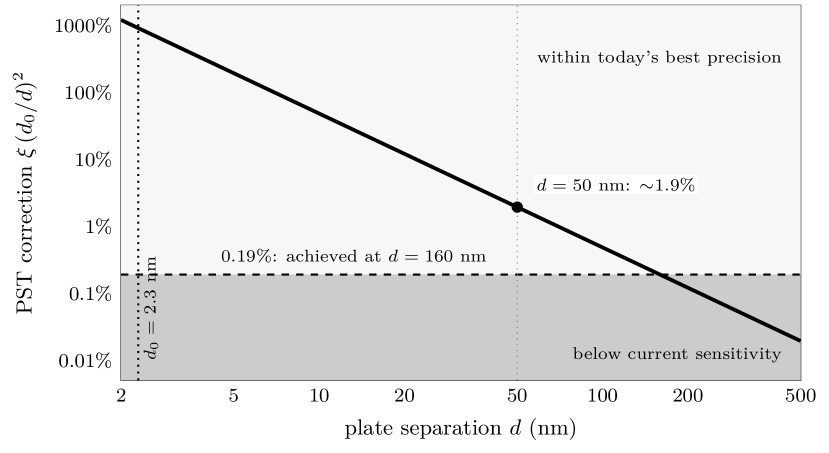
At $d=160$ nm, the shortest separation of the existing precision measurements [212]:

$$\left.\left(\frac{d_{0}}{d}\right)^{\!2}\right|_{d=160\,\mathrm{nm}}\;=\;\left(\frac{2.3}{160}\right)^{2}\;\approx\;2.07\times 10^{-4}$$ (209)

The PST correction with $\xi=90/\pi^{2}$ is $9.12\times 0.0208\%\approx 0.19\%$. This sits right at the measured precision floor at that separation, $0.19\%$ at $95\%$ confidence [212]; the theory is consistent with existing data, and a coherence length larger than the bound would already have shown up there.

At $d=50$ nm, accessible to torsion-pendulum and AFM-based Casimir experiments currently under development:

$$\left.\left(\frac{d_{0}}{d}\right)^{\!2}\right|_{d=50\,\mathrm{nm}}\;=\;\left(\frac{2.3}{50}\right)^{2}\;\approx\;2.13\times 10^{-3}$$ (210)

The correction with $\xi=90/\pi^{2}$ is $9.12\times 0.213\%\approx 1.9\%$, an order above the $0.19\%$ floor already achieved at $160$ nm; it would be detectable if that precision were carried down to $50$ nm and $d_{0}$ sat at its bound, which under the canonical normalisation it does not.

At $d=20$ nm, near the practical lower limit for parallel-plate measurements:

$$\left.\left(\frac{d_{0}}{d}\right)^{\!2}\right|_{d=20\,\mathrm{nm}}\;=\;\left(\frac{2.3}{20}\right)^{2}\;\approx\;0.0133$$ (211)

A correction of $9.12\times 1.33\%\approx 12\%$ over standard quantum field theory (QFT) would be unambiguous at the bound: it would exceed finite conductivity corrections (typically $2$–$5\%$ at these separations), surface roughness corrections ($\lesssim 1\%$ for well-prepared surfaces), and thermal corrections (subdominant below $100$ nm at room temperature [15]).

The distinguishing experimental signature throughout is the power law: standard QFT and all known material corrections modify the coefficient of $d^{-4}$ or introduce $d^{-3}$ thermal terms, while none contribute at order $d^{-6}$, so the $d^{-6}$ PST term is separable by fitting measurements at multiple separations and its ratio to the $d^{-4}$ term grows as separation decreases (the categorical-exponent and two-layer-falsifiability structure is established in §15.6). Substituting the diagnostic upper bound $d_{0}\approx 2.3$ nm explicitly into equation (208):

$$\delta P_{\mathrm{PST}}(d)\;=\;-\frac{\xi\,\pi^{2}\hbar c\times(2.3\;\mathrm{nm})^{2}}{240\,d^{6}}$$ (212)

The coefficient $\xi=90/\pi^{2}\approx 9.12$ is derived exactly from the Gaussian moments of the substrate weight function; see equation (213). Measuring the $d^{-6}$ component at two separations via the ratio test (218) would determine the amplitude scale $d_{0}$ from the data, with $\xi=90/\pi^{2}$ fixed by the theory, and compare it with the value $2.2$ am the normalisation premise fixes; measurements at additional separations overconstrain that one scale, providing an internal consistency check on the $d^{-6}$ form.

15.6.  The parameter-free exponent and falsifiability

A careful reader will observe that equation (208) contains two quantities whose precise values determine the amplitude: the coefficient $\xi$ and the scale $d_{0}$. The situation is as follows.

The discreteness scale $d_{0}$ is the Landau–Ginzburg coherence length; its value is set by the LG vacuum structure and is not pinned by the three foundational postulates alone. The coefficient $\xi$, by contrast, is determined exactly by the Gaussian moments of the PST projection kernel $K$:

$$\xi\;=\;\frac{15}{\pi^{2}}\,\frac{\displaystyle\int_{0}^{\infty}e^{-x^{2}/(4d_{0}^{2})}\,x^{4}\,dx}{\displaystyle d_{0}^{2}\int_{0}^{\infty}e^{-x^{2}/(4d_{0}^{2})}\,x^{2}\,dx}\;=\;\frac{15}{\pi^{2}}\times 6\;=\;\frac{90}{\pi^{2}}\;\approx\;9.12,$$ (213)

Dimensional verification: $\xi$ is a pure number. Substituting $u=x/(2d_{0})$ evaluates the integrals exactly:

$$\int_{0}^{\infty}e^{-x^{2}/(4d_{0}^{2})}\,x^{4}\,dx\;=\;12\sqrt{\pi}\,d_{0}^{5},\qquad\int_{0}^{\infty}e^{-x^{2}/(4d_{0}^{2})}\,x^{2}\,dx\;=\;2\sqrt{\pi}\,d_{0}^{3}.$$ (214)

Hence the numerator carries dimension $d_{0}^{5}$ (length⁵) and the denominator carries $d_{0}^{2}\times d_{0}^{3}=d_{0}^{5}$ (length⁵), so the ratio is dimensionless: $12\sqrt{\pi}\,d_{0}^{5}/(d_{0}^{2}\times 2\sqrt{\pi}\,d_{0}^{3})=6$, and $\xi=15\times 6/\pi^{2}=90/\pi^{2}$. The $d_{0}^{2}$ in the denominator of equation (213) is not “dangling”: it is the factor that cancels the $d_{0}^{5}$ from the $x^{4}$ moment against the $d_{0}^{3}$ from the $x^{2}$ moment, leaving a pure number. This cancellation was verified symbolically (Computations 68, 73).

The coefficient $\xi=90/\pi^{2}\approx 9.12$ is therefore fixed exactly given the Gaussian kernel choice; the amplitude $\xi\,d_{0}^{2}$ is parameter-free in its coefficient, with the scale $d_{0}$ the Landau–Ginzburg coherence length.

15.6.1.  Kernel-shape sensitivity and the $d_{0}$ bound

The numerical value $\xi=90/\pi^{2}$ is conditional on the Gaussian projection-kernel form. Computation 68 (Appendix B) tests the sensitivity of $\xi$ across six plausible alternative kernel shapes, Gaussian, squared Lorentzian, single-sided exponential, hyperbolic-secant-squared, compact parabolic, and compact quartic-bump, by evaluating the moment ratio $M_{4}/(d_{0}^{2}M_{2})$ for each. Findings:

• The $d^{-6}$ power-law exponent is preserved across every kernel tested. This is expected from the structural derivation above (parity plus the existence of a single length scale $d_{0}$), but Computation 68 confirms it numerically and isolates the kernel-dependence to the coefficient $\xi$ alone.

• The coefficient $\xi$ varies by approximately a decade across the kernel family. Concretely: $\xi_{\mathrm{Gaussian}}=9.12$; $\xi_{\mathrm{exp}}=18.2$; $\xi_{\mathrm{sech}^{2}}=21.0$; $\xi_{\mathrm{compact\;quartic}}=2.0$; $\xi_{\mathrm{compact\;parabolic}}=2.6$; $\xi_{\mathrm{Lorentzian}}=378.7$ (the Lorentzian outlier is from the $1/x^{4}$ heavy tail, which is physically implausible for a substrate discreteness scale). Restricting to the four kernels with exponential or compact-support tails, the range is $\xi\in[2,21]$, a factor of $\sim 10$.

• The diagnostic $d_{0}$ bound from current nanometre-Casimir data scales as $1/\sqrt{\xi}$. Under the same data, the kernel-conditional bound ranges from $d_{0}\lesssim 1.5$ nm (sech²) to $d_{0}\lesssim 4.9$ nm (compact quartic), with the Gaussian value $d_{0}\lesssim 2.3$ nm between them. The order of magnitude (a few nm) is robust; the precise numerical bound is kernel-conditional with a factor-of-$\sim 3$ spread.

The honest reading is therefore: the $d^{-6}$ signature is parameter-free and falsifiable; the amplitude $\xi d_{0}^{2}$ that converts a measured deviation into an inferred $d_{0}$ carries a kernel-shape systematic of order a factor of two to three on $d_{0}$. Reports of the bound should read “$d_{0}\lesssim 1.5$–$5$ nm depending on the projection-kernel choice; the Gaussian (canonical) choice gives $2.3$ nm.” See Computation 68 for the full kernel table.

15.6.2.  The Gaussian as the substrate’s kernel

The kernel-shape sensitivity above frames $\xi$ as conditional on a choice of kernel. Computation 73 sharpens this by deriving the substrate’s actual projection kernel directly from its Boolean structure and showing it is asymptotically Gaussian, with a calculable non-Gaussian correction that vanishes at the matched scaling. The substrate Hilbert space $\mathbb{C}^{2^{D}}$ carries the Boolean kernel $K_{n}(j)=\binom{n}{j}\,(1/2)^{n}$, the binomial distribution at $p=1/2$ (the per-site Bernoulli probability of $\mu=\bigotimes_{a\in D}\mathrm{Bern}(1/2)$). By the central limit theorem (CLT), the binomial converges to a Gaussian as $|D|\to\infty$ at the matched scaling. The leading-order non-Gaussian correction is in the kurtosis:

$$\mathrm{kurt}(\mathrm{binomial}|_{p=1/2})\;=\;3-\frac{2}{|D|},\qquad\mathrm{kurt}(\mathrm{Gaussian})\;=\;3.$$ (215)

Substituting into the moment ratio $M_{4}/M_{2}^{2}$ that fixes $\xi$ gives

$$\xi_{\mathrm{substrate}}(|D|)\;=\;\xi_{\mathrm{Gaussian}}\cdot\left(1-\frac{2}{3\,|D|}\right)\;=\;\frac{90}{\pi^{2}}\,\left(1-\frac{2}{3\,|D|}\right).$$ (216)

The kernel-shape conditional of Computation 68 is therefore not arbitrary: the substrate is approximately Gaussian by CLT, with the leading correction $-2/(3|D|)$ a small downward shift that vanishes at the matched scaling. At $|D|=6$ the correction is $11\%$; at $|D|=20$, $3.3\%$; at $|D|=100$, less than $1\%$. The diagnostic $d_{0}\lesssim 2.3$ nm bound derived from the Gaussian value is therefore correct to leading order; the substrate’s actual bound is shifted by at most a few percent at any physically relevant $|D|$. This converts the kernel-shape conditional from “$\xi$ depends on a choice of kernel” to “$\xi$ is structurally Gaussian with a calculable convergence rate”.

What does not depend on $\xi$ or $d_{0}$ is the power-law exponent. As derived above for equation (208), the exponent $-6$ follows from the parity constraint and the existence of a single length scale $d_{0}$ alone, and uses neither the value of $\xi$ nor of $d_{0}$. Odd powers of $d_{0}/d$ would require a preferred substrate orientation, inconsistent with the isotropy of Chapter 4. The exponent $-6$ is therefore a categorical prediction: it cannot be changed by adjusting $\xi$ upward or downward, by moving $d_{0}$ within its allowed range, or by any other parametric variation within the theory.

The experimental consequence is that the test of PST’s Casimir prediction has two logically distinct layers. The first layer is qualitative and parameter-free: does the measured Casimir pressure, after subtracting the Lifshitz-theory prediction (which already accounts for finite conductivity, surface roughness, and thermal fluctuations to high precision), show a residual that scales as $d^{-6}$? If the residual is consistent with zero within experimental uncertainty, PST is constrained. If it shows a different power law that cannot be attributed to known corrections, PST is falsified. A $d^{-6}$ residual is a necessary condition for PST at this order, but not sufficient: other single-length-scale modifications of the vacuum also predict $d^{-6}$ [15]. At the first layer PST therefore makes a categorical prediction about the form of the correction (the exponent), not about its amplitude.

The second layer, conditioned on observing $d^{-6}$ scaling, is quantitative. $\xi=90/\pi^{2}$ is fixed exactly by the projection-kernel moments. The amplitude $\xi d_{0}^{2}$ contains one further quantity, $d_{0}$, the Landau–Ginzburg coherence length, which P1–P3 alone do not fix: it follows from the canonical normalisation of §12.2, the premise on which $M_{*}$ rests, as $d_{0}=\sqrt{2}\,\hbar c/m_{h}=2.2$ am (Computation 201). Existing $160$–$750$ nm precision Casimir data constrain $d_{0}$ only by an upper bound, $d_{0}\lesssim 2.3$ nm (equation (217) at the derived $\xi=90/\pi^{2}$), nine orders above that value. A measured residual at $d^{-6}$ with amplitude $A$ would therefore determine $d_{0}=\sqrt{A/\xi}$ from the data, and any resolvable amplitude would put it far above $2.2$ am and refute the normalisation rather than confirm the book. Inconsistency between the inferred $d_{0}$ from different experimental separations would falsify PST at the second layer; a single amplitude measurement at the precision required to extract a $d^{-6}$ residual constitutes a determination of $d_{0}$, not a sharp test.

Honest comparison with parameter-rigid tests: the gravitational-wave tests of General Relativity constrain a specific waveform morphology in which both the exponent (post-Newtonian structure) and the amplitude (Bayesian fit to source parameters) are predicted up to a finite list of source-parameter inputs (masses, spins). PST’s Casimir test is exponent-rigid, and since the normalisation premise fixed $d_{0}$ (Computation 201) it is amplitude-rigid as well, on that premise: the exponent layer is parameter-free, and the amplitude layer is a prediction conditional on the canonical normalisation rather than a fit. The asymmetry that remains is between a structural consequence and a carried premise, and §12.2 names the premise.

The $d^{-6}$ scaling is separable from the standard $d^{-4}$ Casimir dependence by fitting measurements at multiple separations. The correction budget at relevant separations is discussed in detail in §15.9. In brief: finite-conductivity corrections enter via the Lifshitz formula [17] as an effective $d^{-5}$ correction at leading order in $\lambda_{\mathrm{plasma}}/d$, and this Lifshitz-corrected Casimir force is well-known and can be subtracted with high precision. The PST $d^{-6}$ signal would appear as a residual after this subtraction. Surface roughness introduces corrections at the spatial-frequency scale of the roughness spectrum, with a known power-law dependence; thermal corrections have a distinct temperature dependence isolable by varying plate temperature. The subtraction strategy is the standard one used in current precision Casimir experiments [15]; the challenge is the accuracy required to resolve a ${\sim}2\%$ residual at $d=50$ nm after subtracting Lifshitz corrections that are themselves of order 100% at this separation.

15.7.  Falsifiability and the experimental programme

The PST Casimir prediction satisfies strict experimental falsifiability, with the two-layer structure of §15.6: the $d^{-6}$ exponent is the parameter-free content, while the amplitude carries the onset scale $d_{0}$, fixed by the normalisation premise at $2.2$ am and bounded by the data at $2.3$ nm. The prediction is refuted if:

1. A non-$d^{-6}$ short-distance power law is detected, inconsistent with PST’s even-in-$d_{0}/d$ expansion (any power law intermediate between $d^{-4}$ and $d^{-6}$ would falsify the theoretical structure, not merely constrain $d_{0}$).

Null results, by contrast, tighten the bound on $d_{0}$ without refuting the structure, and they are what the theory expects at every reachable precision. Agreement with standard QFT to better than $1\%$ at $d=50$ nm would constrain $d_{0}<1.7$ nm, still nine orders above the derived value. Multi-separation ratio tests (equation (218)) in the $20$–$50$ nm range, finding no $d^{-6}$ component at the $0.5\%$ level, would push the bound lower still. A $d^{-6}$ component resolved at any reachable amplitude would confirm the form and refute the normalisation premise; the following would establish the form:

1. A $d^{-6}$ component is detected at separations below $50$ nm, with amplitude consistent with $d_{0}\lesssim 2.3$ nm.

2. The ratio test between separations $d_{1}\approx 20$ nm and $d_{2}\approx 160$ nm yields $(d_{0}/d_{1})^{2}-(d_{0}/d_{2})^{2}$ consistent with that same $d_{0}$.

3. The fitted $d_{0}$ is stable across separations, apparatus, and materials: a single onset scale accounts for every ratio test, as a single Landau–Ginzburg coherence length requires.

Current experiments [212, 15] at $160$–$750$ nm agree with standard QFT to $0.19\%$ at $160$ nm, consistent with $d_{0}<7.0\,\mathrm{nm}/\sqrt{|\xi|}$ from equation (217), i.e. $d_{0}\lesssim 2.3$ nm at the derived $\xi=90/\pi^{2}$. The onset scale $d_{0}=2.2$ am the normalisation premise fixes lies nine orders below this bound, so current Casimir data are consistent with it and no planned experiment reaches the predicted amplitude; what the next generation of sub-$50$ nm measurements can do is lower the data’s bound.

As established in §15.6, the $d^{-6}$ exponent and the coefficient $\xi=90/\pi^{2}$ are structural, while the onset scale $d_{0}$ is the Landau–Ginzburg coherence length. A measured $d^{-6}$ residual at sub-$50$ nm separations would support the substrate-discreteness prediction, and a short-distance power law measured inconsistent with $d^{-6}$ would falsify it. A null result, by contrast, only tightens the data’s bound on $d_{0}$, whose value the normalisation premise fixes far below it. The modal scale $M_{*}=4\pi m_{h}\sqrt{2/3}\approx 1.285$ TeV is a separate, collider-testable prediction: PST expects new physics associated with the modal condensate near this scale. The substrate Walsh zero mode maps under the projection chain $\psi\to\Pi(\psi)\to H_{\mathrm{doublet}}$ to the constant function on $M$ (vacuum direction), structurally distinct from the emergent SM Higgs doublet generated by inner fluctuations on $M\times F$ (Computations 93 and 97). With that distinction explicit, the scalar-sector cancellation closes and $M_{*}=4\pi m_{h}\sqrt{2/3}$ is a parameter-free one-loop derivation of the scalar sector on the canonical normalisation (§12.2); its full-SM extension is settled in the negative (Computation 120).

15.8.  Observational constraint on $d_{0}$ from Casimir data

Precision Casimir measurements at separations $160$–$750\;\mathrm{nm}$ [212] report $0.19\%$ agreement with standard QFT at $160$ nm, at $95\%$ confidence [212, 15]. Requiring $|\xi|(d_{0}/d)^{2}<1.9\times 10^{-3}$ at $d=160\;\mathrm{nm}$ gives:

$$d_{0}\;<\;\frac{160\;\mathrm{nm}\,\sqrt{1.9\times 10^{-3}}}{\sqrt{|\xi|}}\;\approx\;\frac{7.0\;\mathrm{nm}}{\sqrt{|\xi|}}$$ (217)

With the PST-derived $\xi=90/\pi^{2}\approx 9.12$ (conditional on the Gaussian convolution-kernel form; §15.6), this constrains $d_{0}\lesssim 2.3\;\mathrm{nm}$. The PST correction sits at that $0.19\%$ precision for separations $d\lesssim 69\,d_{0}$ (where $|\xi|(d_{0}/d)^{2}\geq 1.9\times 10^{-3}$ at $\xi=90/\pi^{2}$), which at the bound is $d\lesssim 160\;\mathrm{nm}$, the precision of existing measurements; it reaches the $1\%$ level for $d\lesssim 30\,d_{0}\approx 70\;\mathrm{nm}$. A ratio test between measurements at two separations $d_{1}$ and $d_{2}$ provides a clean, apparatus-independent signature:

$$\frac{P(d_{1})/P_{\mathrm{standard}}(d_{1})}{P(d_{2})/P_{\mathrm{standard}}(d_{2})}-1\;\propto\;\left(\frac{d_{0}}{d_{1}}\right)^{\!2}-\left(\frac{d_{0}}{d_{2}}\right)^{\!2}$$ (218)

This represents a falsifiable prediction distinguishable from both standard QFT and Lifshitz-theory corrections.

What the theory fixes without free parameters is the form of the correction: the $d^{-6}$ scaling and the coefficient $\xi=90/\pi^{2}\approx 9.12$ (equation (213)). The overall amplitude scales as $(d_{0}/d)^{2}$, with $d_{0}$ the Landau–Ginzburg coherence length of the modal condensate (§15.3). Its magnitude is fixed by the canonical normalisation at $2.2$ am (Computation 201), seventeen orders above $\ell_{P}$ and nine below the diagnostic bound. The budget below is evaluated at the bound, $d_{0}=2.3$ nm, where the correction is at the edge of current precision near $d=160\;\mathrm{nm}$, reaches several percent near $d=50\;\mathrm{nm}$ and $12$ percent at $d=20\;\mathrm{nm}$; that is the sensitivity a measurement would have, not the signal the theory expects, which at the derived $d_{0}$ is $10^{-19}$ of the force at $20$ nm.

15.9.  Correction budget for the Casimir measurement

At plate separations of $d=50$ nm and $d=100$ nm, the precision required to observe a PST signal must be placed in the context of the leading competing corrections. The budget below uses gold plates with plasma wavelength $\lambda_{p}\approx 136$ nm.

Correction	Relative size at $50\;\mathrm{nm}$	Relative size at $100\;\mathrm{nm}$
Standard Casimir ($d^{-4}$)	$1$ (reference)	$1$
Finite conductivity (Lifshitz, $\sim\lambda_{p}/d$)	$\sim 270\%$	$\sim 136\%$
Surface roughness ($\sim\sigma^{2}/d^{2}$ for rms $\sigma\approx 1$ nm)	$\sim 0.04\%$	$\sim 0.01\%$
Thermal/Lifshitz ($k_{B}Td/\hbar c$, at 300 K)	$\sim 0.5\%$	$\sim 1.0\%$
PST $d^{-6}$ at $d_{0}=2.3$ nm (upper bound)	$\mathbf{\sim 1.9\%}$	$\mathbf{\sim 0.48\%}$
PST $d^{-6}$ at $d_{0}=1.1$ nm	$\sim 0.44\%$	$\sim 0.11\%$

The dominant correction at small separations is the finite-conductivity Lifshitz term, which at $d=50$ nm is larger than the standard Casimir force itself; it does not, however, mimic a $d^{-6}$ power law. The Lifshitz formula with the measured optical data of the plate material predicts this correction to better than 1% accuracy [15, 17] and can be subtracted. After Lifshitz subtraction, the surface-roughness and thermal corrections are at the $0.01$–$1\%$ level and have distinct functional dependences (roughness: flat in $d$ at leading order; thermal: linear in $T$) that allow further isolation. The PST $d^{-6}$ signal is then the residual. At the diagnostic upper bound $d_{0}\approx 2.3$ nm, the correction is ${\sim}1.9\%$ at $d=50$ nm, an order above the $0.19\%$ precision already achieved at $160$ nm and robustly detectable if that precision is carried down to $50$ nm.

15.9.1.  Predicted deviation across separations

The fractional deviation from the standard Casimir force is $\delta F/F=\xi\,(d_{0}/d)^{2}$ with the parameter-free coefficient $\xi=90/\pi^{2}\approx 9.12$; the amplitude-setting $d_{0}$ is $2.2$ am under the normalisation premise and is bounded by the data at $d_{0}\lesssim 2.3$ nm, the value the table is evaluated at. Table 1 gives the predicted deviation across the experimentally relevant separations and three representative coherence lengths. Boldface entries exceed the $0.19\%$ floor achieved at $160$ nm by the micromechanical torsional oscillator of [212] and are detectable if that precision is carried to the separation in question; the remainder are next-generation targets. Because the deviation scales as $d^{-2}$ relative to the standard force while the systematics tabulated above carry distinct functional forms, the two-separation ratio test (equation (218)) isolates the $d^{-6}$ component apparatus-independently.

Table 1: PST predicted fractional Casimir deviation $\delta F/F=\xi\,(d_{0}/d)^{2}$ (coefficient $\xi=90/\pi^{2}\approx 9.12$ parameter-free; amplitude set by $d_{0}$) versus plate separation $d$ and coherence length $d_{0}$. Boldface entries exceed the $0.19\%$ precision achieved at $160$ nm [212]. The dominant systematic (finite-conductivity Lifshitz) is $d^{-1}$-like and subtractable to $<1\%$ from optical data; roughness ($\sim\sigma^{2}/d^{2}$) and thermal ($\sim k_{B}Td/\hbar c$) corrections sit at $0.01$–$1\%$ with distinct $d$-dependences.

$d$ (nm)	$d_{0}=0.5$ nm	$d_{0}=1.1$ nm	$d_{0}=2.3$ nm
$20$	$\mathbf{0.57\%}$	$\mathbf{2.8\%}$	$\mathbf{12\%}$
$30$	$\mathbf{0.25\%}$	$\mathbf{1.2\%}$	$\mathbf{5.4\%}$
$50$	$0.09\%$	$\mathbf{0.44\%}$	$\mathbf{1.9\%}$
$100$	$0.02\%$	$0.11\%$	$\mathbf{0.48\%}$
$160$	$0.01\%$	$0.04\%$	$0.19\%$

15.10.  Experimental status of $M_{*}$ and the ADD comparison

PST is superficially analogous to the ADD model [16] only in involving structure beyond the four macroscopic dimensions. The full operator-by-operator Standard Model effective field theory (SMEFT) survey of empirical $M_{*}$ bounds against LHC and electroweak precision observables (EWPO) is carried out in Computation 10, with the tree-level custodial $\mathrm{SU}(2)$ protection of $\Delta T$ confirmed at $\Delta T=0$ (loop and new-states corrections to $S$ and $T$ are not computed there). A critical difference makes ADD collider and astrophysical bounds inapplicable to PST: the additional structure is a finite noncommutative internal factor, not large extra spatial dimensions, and its only associated length is the sub-fermi modal scale $\ell_{*}=\hbar c/M_{*}\approx 1.535\times 10^{-19}$ m, far from the millimetre-to-micron range ADD requires for its gravity-dilution mechanism. The ADD bounds on the fundamental scale (LHC mono-jet/mono-photon ($M_{*}\gtrsim 5$–$8$ TeV), SN1987A and neutron-star Kaluza–Klein (KK) graviton emission) are all derived for macroscopic extra dimensions, with KK gravitons coupling to the full stress-energy tensor at tree level with the four-dimensional Newton constant. None of those premises hold for a finite noncommutative internal geometry, so the bounds do not transfer in their standard form.

What remained until Computation 205 was a genuine empirical-consistency question, not a derived constraint: whether $M_{*}=4\pi m_{h}\sqrt{2/3}\approx 1.285$ TeV (a parameter-free one-loop derivation; Computations 93, 97) is consistent with the existing data once the PST-specific coupling structure (set by the projection operator $\Pi$) is computed. Computation 205 performs it under the three readings this book’s sentences admit of what $M_{*}$ does to the fields below it. Read literally, as a momentum cutoff above which no field mode exists, it predicts no event with a parton momentum above $1.285$ TeV; the ATLAS experiment measures dijet masses to $9$ TeV and jet transverse momenta to $3.5$ TeV with next-to-next-to-leading-order quantum chromodynamics (QCD) describing them [217], and holds $25$ dilepton events above $2$ TeV where the Standard Model expects $22$ [218], so that reading is excluded outright. Read as the projection’s Gaussian kernel on every vertex, it multiplies the Drell–Yan yield above $2.2$ TeV by $0.05$ against $19$ observed dielectron events, and its linearised form is a contact interaction with an equivalent scale of $13$ to $16$ TeV against the published limits of $32$ to $36$ TeV [218], short by a factor five in $1/\Lambda^{2}$; a universal kernel would have to sit at $2.7\,M_{*}$ or above. Read as the kernel on the Higgs doublet alone, the field that is the projected condensate (§15.2), everything measured is consistent: the coupling modifiers shift by half a percent against $\kappa_{V}=1.035\pm 0.031$ and $\kappa_{F}=0.95\pm 0.05$ [219]; Higgs production above $450$, $650$ and $1000$ GeV of transverse momentum is suppressed by $12$, $23$ and $45$ percent against measurements whose uncertainties are of order the value [221]; Higgs pairs are suppressed by $27$ percent against a limit of $2.4$ times the Standard Model [220]; and because the whole doublet carries the kernel, Goldstones included, the cancellation that keeps longitudinal vector-boson scattering bounded is preserved, consistent with the measured same-sign $WW$ rate [222], where a kernel on the physical $h$ alone would break the partial-wave bound at $1.5$ TeV. The surviving reading is the one §12.2 now states, and it predicts: a deficit in the Higgs transverse-momentum spectrum growing as $1-\mathrm{e}^{-p_{T}^{2}/M_{*}^{2}}$, $23$ percent above $650$ GeV, within the reach of the high-luminosity run. The first measurement in that bin, ATLAS’s boosted $H\to\tau\tau$ on Run 2 plus partial Run 3 [234], gives a Run 2 deficit above $650$ GeV and a combined upper limit of $4.5$ times the Standard Model at $95\%$ confidence: a limit, not yet the measurement at $15$ percent precision that would decide it, so the exposure stands untested. The coherence length $d_{0}$ that sets the absolute size of the Casimir signal is fixed by the canonical normalisation at $2.2$ am (Computation 201), so the signal is predicted in form (the $d^{-6}$ scaling and the coefficient $\xi=90/\pi^{2}$) and in size, far below present reach (§15.5).

15.11.  Wilson coefficients: tree-level custodial $\Delta T$ protection

PST’s structural commitments fix the dim-6 SMEFT Wilson coefficients that control the electroweak $S$ and $T$ parameters to zero exactly, so PST contributes no new-physics correction to the global electroweak fit (Computation 10, section 10 of the script).

The argument is structural. PST’s Landau–Ginzburg modal potential $V(H^{\dagger}H)=-\varepsilon\,(H^{\dagger}H)+\tfrac{1}{4}(H^{\dagger}H)^{2}$ is a function of the $\mathrm{SU}(2)_{L}\times\mathrm{SU}(2)_{R}$ singlet $H^{\dagger}H$ only; it is manifestly custodial-symmetric. The dim-6 operators $\mathcal{O}_{HWB}=(H^{\dagger}\sigma^{a}H)W^{a\mu\nu}B_{\mu\nu}$ and $\mathcal{O}_{HD}=(H^{\dagger}D_{\mu}H)^{\dagger}(H^{\dagger}D^{\mu}H)$ are the unique custodial-breaking dim-6 operators that mix the $\mathrm{SU}(2)_{L}$ triplet of $W$ with $B$ and that modify the Higgs kinetic term respectively. Their coefficients $c_{\mathrm{HWB}}$ and $c_{\mathrm{HD}}$ encode the amount of custodial breaking induced by integrating out heavy modes above the matching scale. Since PST’s substrate adds no custodial-breaking new physics above $M_{*}$ (the LG potential is custodial-symmetric, and the substrate modes integrated out between any $\mu$ and $M_{*}$ are higher harmonics of $H$ itself), the matching-scale Wilson coefficients are $c_{\mathrm{HWB}}(M_{*})=c_{\mathrm{HD}}(M_{*})=0$, exactly.

Consequently the PST contribution to the Peskin–Takeuchi parameters is

$$\Delta S_{\mathrm{PST}} =(16\sin\theta_{W}\cos\theta_{W}/\alpha_{\mathrm{em}})\cdot v^{2}/M_{*}^{2}\cdot c_{\mathrm{HWB}}(M_{*})=0,$$ (219)

$$\Delta T_{\mathrm{PST}} =0.$$

The SM-internal contributions to $S$ and $T$ (top quark, gauge-Higgs loops) are part of the SM reference prediction that the Particle Data Group (PDG) 2024 fit measures against; they are not “PST corrections”. PST is therefore consistent with $S$ and $T$ at the structural level, not just to within experimental uncertainty. The bounds $|\Delta S|<0.20$, $|\Delta T|<0.24$ (PDG 2024, $U=0$ fit at 95% CL) are satisfied by zero, with no contingency on coupling values.

Other SMEFT operators are pushed to loop level by PST’s structural commitments at the level of the established content (no new gauge bosons, no new light fermions, the substrate modes being higher harmonics of the Higgs). The hypothetical Boolean partner states that a full-SM boson–fermion cancellation at $M_{*}$ would require (§12.2) are not part of this demonstrated content. That cancellation is settled in the negative (Computation 120), with §19.9.6 recording the closure, and the light-EFT conclusions here are unaffected. Four-fermion contact operators $(\bar{\psi}\gamma_{\mu}\psi)(\bar{\psi}\gamma^{\mu}\psi)$ require new vector or scalar mediators, which PST lacks, so their tree-level Wilson coefficients vanish. The loop-suppressed values give effective scales $\Lambda_{\mathrm{eff}}=M_{*}/\sqrt{c}\approx 30$ TeV, at the current LHC Drell–Yan high-mass bound of $32$ to $36$ TeV [218]; in the reading of the cutoff that survives Computation 205 the gauge vertices carry no kernel at all, so four-fermion operators arise only through doublet exchange, Yukawa-suppressed, and sit far above the bound, while a kernel on the gauge vertices themselves is what the same data exclude. Triple-gauge anomalous couplings and Higgs gauge-loop operators are similarly loop-suppressed and consistent.

The astrophysical bounds (SN1987A neutron-star cooling, and large-extra-dimension graviton emission) do not transfer to PST, for the reason given in §15.10. PST has no Kaluza–Klein tower: the internal factor $F$ is a finite noncommutative geometry with sub-fermi associated length, not a set of macroscopic extra dimensions.

The empirical consistency question raised earlier in this section is therefore settled by Computation 205 rather than by construction: $M_{*}=4\pi m_{h}\sqrt{2/3}\approx 1.285$ TeV is not in tension with any existing collider or astrophysical bound in the Higgs-doublet reading of the cutoff, which is the one §15.2 states, and it is excluded by existing data in the two readings that would put the kernel on the emergent quanta.

15.12.  Summary

This chapter derives the Casimir signature of the substrate and assesses its experimental reach. Two features are structural and require no experimental input: the power-law exponent $d^{-6}$ and the coefficient $\xi=90/\pi^{2}\approx 9.12$, the latter derived exactly from the Gaussian moments of the substrate weight function (and kernel-shape sensitive: a factor-of-$\sim 10$ spread in $\xi$ across plausible kernel families, Computation 68, becomes a factor-of-$\sim 3$ spread in the bound inferred from it), together with the functional separability of the signal from competing effects (Lifshitz, thermal, roughness). The absolute amplitude scales as $(d_{0}/d)^{2}$ and is therefore set by the coherence length $d_{0}$ of the modal condensate, which the canonical normalisation fixes at $2.2$ am (Computation 201); the electroweak modal scale is $M_{*}=4\pi m_{h}\sqrt{2/3}\approx 1285\;\mathrm{GeV}$ from $m_{h}$ alone. At the diagnostic upper bound $d_{0}\approx 2.3\;\mathrm{nm}$ the correction would be ${\sim}1.9\%$ at $50\;\mathrm{nm}$ and ${\sim}12\%$ at $20\;\mathrm{nm}$, within reach of next-generation precision Casimir experiments; at the derived $d_{0}$ it is $10^{-19}$ of the force at $20$ nm, and a null result at every reachable precision is what the theory expects.

On the status of $d_{0}$: as grounded in §15.3, it is the Landau–Ginzburg coherence length of the modal condensate, $d_{0}=\xi_{\psi}=\sqrt{c_{\scriptscriptstyle LG}/(2|a_{\scriptscriptstyle LG}|)}$, not the substrate’s microscopic grain. Its magnitude is not an output of P1–P3 alone: with $|a_{\scriptscriptstyle LG}|=m_{h}^{2}/4$ it is the gradient normalisation in another variable, and the canonical normalisation on which $M_{*}$ rests puts it at $\sqrt{2}\,\hbar c/m_{h}=2.2$ am (Computation 201).